Finite Volume Techniques
B.1Introduction
Inverse problems are common across the geosciences: for example, in geophysical imaging, history matching, and parameter estimation. Many of these inverse problems require constrained optimization using partial differential equations (PDEs), which requires derivatives with respect to mesh variables in addition to simulation of the PDE. Finite difference, finite element, and finite volume techniques allow subdivision of continuous differential equations into discrete domains. Knowledge and the appropriate application of these methods is fundamental to simulating physical processes. Many inverse problems in the geosciences are solved using stochastic techniques or external finite difference-based tools (e.g. Doherty (2004)), which are robust to local minima and the programmatic implementation, respectively. However, these methods do not scale to situations where millions of parameters are to be estimated. This sort of scale is necessary for solving many of the inverse problems in geophysics and, increasingly, hydrogeology (e.g. electromagnetics, gravity, and fluid flow problems).
In the context of the inverse problem, when the physical properties, the domain, and the boundary conditions are not necessarily known, the simplicity and efficiency in mesh generation are important criteria. Complex mesh geometries, such as body fitted grids, commonly used when the domain is explicitly given, are less appropriate. Additionally, when considering the inverse problem, it is important that operators and their derivatives are accessible for interrogation and extension. The goal of this work is to provide a high-level background to finite volume techniques, which are abstracted across four mesh types: (1) tensor product mesh; (2) cylindrically symmetric mesh; (3) logically rectangular, non-orthogonal mesh; and (4) octree and quadtree meshes. This work contributes an overview of finite volume techniques, in the context of geoscience inverse problems, which are treated in a consistent way across various mesh types in order to highlight similarities and differences.
B.1.1Attribution and dissemination
The numerical implementations underlying this work have been created throughout my PhD in multiple programming languages (i.e. Matlab, Julia, and Python) and have been influenced by course material and instruction from Dr. Eldad Haber, Dr. Uri Ascher and Dr. Chen Grief Haber, 2015Ascher & Greif, 2011. Further references can be found throughout the scientific literature (cf. Yee (1966)Hyman & Shashkov (1999)Hyman & Shashkov (1997)). I have published aspects of this work in Cockett et al. (2015), in many Society of Exploration Geophysics abstracts Heagy et al., 2014Kang et al., 2015Heagy et al., 2015 and in a tutorial paper in The Leading Edge Cockett et al., 2016. Dave Marchant and Lindsey Heagy influenced the development of the cylindrical mesh, and the octree storage algorithm was loosely based on the implementation by Burstedde et al. (2011). These techniques and implementations proved successful in the SimPEG project Cockett et al., 2015 and are used in applications of frequency and time domain electromagnetics, direct current resistivity, gravity, magnetics, fluid flow, and seismic across industry, academia, and education Rosenkjaer et al., 2016Kang & Oldenburg, 2016Heagy et al., 2015Rosenkjaer et al., 2015Cockett et al., 2015Kang et al., 2014.
The techniques discussed below, as well as a number of accompanying utilities for mesh generation, import, export, visualization, documentation, and testing are provided in an open source package for Python, called: discretize (https://discretize package is released using the permissive MIT license to encourage reuse and future improvement of this work. My collaborators and I have also generalized across these types of meshes, in order to have both a high-level and a standard programmatic interface, differing only in mesh instantiation. The generalization of meshes allows both ourselves and others to build upon this work as we continue to improve and expand its capabilities.
B.2Terminology
To simulate differential equations in any computational domain, we must approximate the continuous equations through discretization onto a mesh. The mesh defines boundaries, locations of variables, and connectivity between cells. In this section we will discuss a staggered mimetic finite volume approach Yee, 1966Hyman & Shashkov, 1999Hyman et al., 2002.
B.2.1Mesh types
The topographic interface, the location of boundary conditions, and the location of sources/receivers are often the only non-numerical constraints on mesh generation in geophysics. These constraints require meshes that that can pad efficiently to sufficiently distant boundaries (as in electromagnetics), align or refine to topographic features, and refine around the locations of sources. Numerical efficiency generally translates to minimizing the number of cells used in any computational domain. Here, we will consider four mesh types: (1) tensor product mesh; (2) logically rectangular; non-orthogonal mesh (curvilinear mesh); (3) octree and quadtree meshes; and (4) cylindrically symmetric mesh. We use different techniques for dealing with padding, alignment, and refinement for each mesh. Orthogonal vectors of spacings define a tensor product mesh (tensor mesh). In the 2D example in Figure B.1a, the mesh is created from two vectors, and , which define constant spacing, orthogonal to each direction. As the spacing is fixed, any refinement in one dimension means that that refinement is completed everywhere in the domain. These refinement constraints often lead to meshes with many cells and unnecessary resolution far from the domain of interest. Tree meshes are built through successively dividing mesh cells into four or eight cells in 2D quadtree meshes and 3D octree meshes, respectively (Figure B.1b). Octree meshes are used extensively in electromagnetic geophysical inversions Haber & Heldmann, 2007. These meshes can also be built on a variable tensor spaced grid, but have the advantage of not refining in locations far from areas of interest, resulting in meshes with fewer cells. Unlike the tensor mesh, tree meshes are not logically rectangular; that is, each cell does not necessarily have two neighbours in each dimension (, , , , etc.). A quadtree cell may have additional neighbours if it is coarser than its direct neighbours. Using a mesh leveling algorithm, the level of refinement can be enforced to be a maximum of one level change between cells Burstedde et al., 2011. The tensor mesh is a logically rectangular orthogonal mesh, where 'orthogonal' means that the tensors are orthogonal and define a local Cartesian coordinate system. Another mesh type under consideration is a logically rectangular \emph{non-}orthogonal mesh, where each cell still has two neighbours in each dimension but the cells are neither required to be axes aligned nor to have orthogonal faces. Here, we will refer to logically rectangular non-orthogonal meshes as curvilinear meshes, as seen in Figure B.1c. As these meshes are no longer constrained to have orthogonal cells, topographic layers can be better approximated, without the staircase effect that is present on both tensor and tree meshes. Additionally, curvilinear meshes allow different ways of padding to 'infinity', and can be used to approximate spherical domains Calhoun et al., 2008. Finally, we will also consider a cylindrically symmetric tensor mesh. The cylindrically symmetric tensor mesh is defined in a cylindrical coordinate system where the radial , azimuthal , and vertical dimensions are in the following domains:
Cylindrical symmetry is enforced through a single cell in . With the exception of calculations for boundary conditions, volume and area are formulated similarly to tensor meshes. Cylindrical meshes are often used for electromagnetics problems for layered systems or cylindrically symmetric problems, such as geophysics or fluid flow around a borehole Pidlisecky et al., 2013Heagy et al., 2016. Fully unstructured (tetrahedral) meshes will not be considered here, but are commonly used in geophysics and hydrogeology (e.g. Ollivier-Gooch & Van Altena, 2002Jahandari et al., 2017). We chose the meshes used in this appendix for their common use in electromagnetic geophysics and fluid flow Haber & Ascher, 2001Li & Oldenburg, 1996Egbert & Kelbert, 2012McDonald & Harbaugh, 2003Kelbert et al., 2014Cockett et al., 2015. All meshes are easy to parameterize, which is an advantage when relatively little is known about the simulation domain, as is the case in the context in geophysical inverse problems.
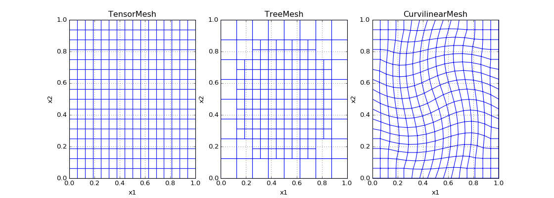
Figure B.1:Three mesh types in two dimensions on the domain of a unit square: (a) a tensor product mesh, (b) a quadtree mesh, and (c) a curviliear mesh.
B.2.2Cell anatomy
This approach requires defining variables at either cell centers, nodes, faces, or edges, as described in Figure B.2. The finite volume technique is derived geometrically from studying the control volume of a mesh 'cell'. The cell center is often used for scalar variables or anisotropic tensors that represent physical properties. This shows that a single value fills the entire cell, allowing discontinuities between adjacent cells. From a geologic perspective, discontinuities are prevalent, as large differences in physical properties may exist between geologic layers. Cell nodes, alternatively, are often used for variables that are continuously varying in space; that is, internal to a cell values between nodes can be found through bi/tri-linear interpolation. Vector quantities are held on the faces or edges.
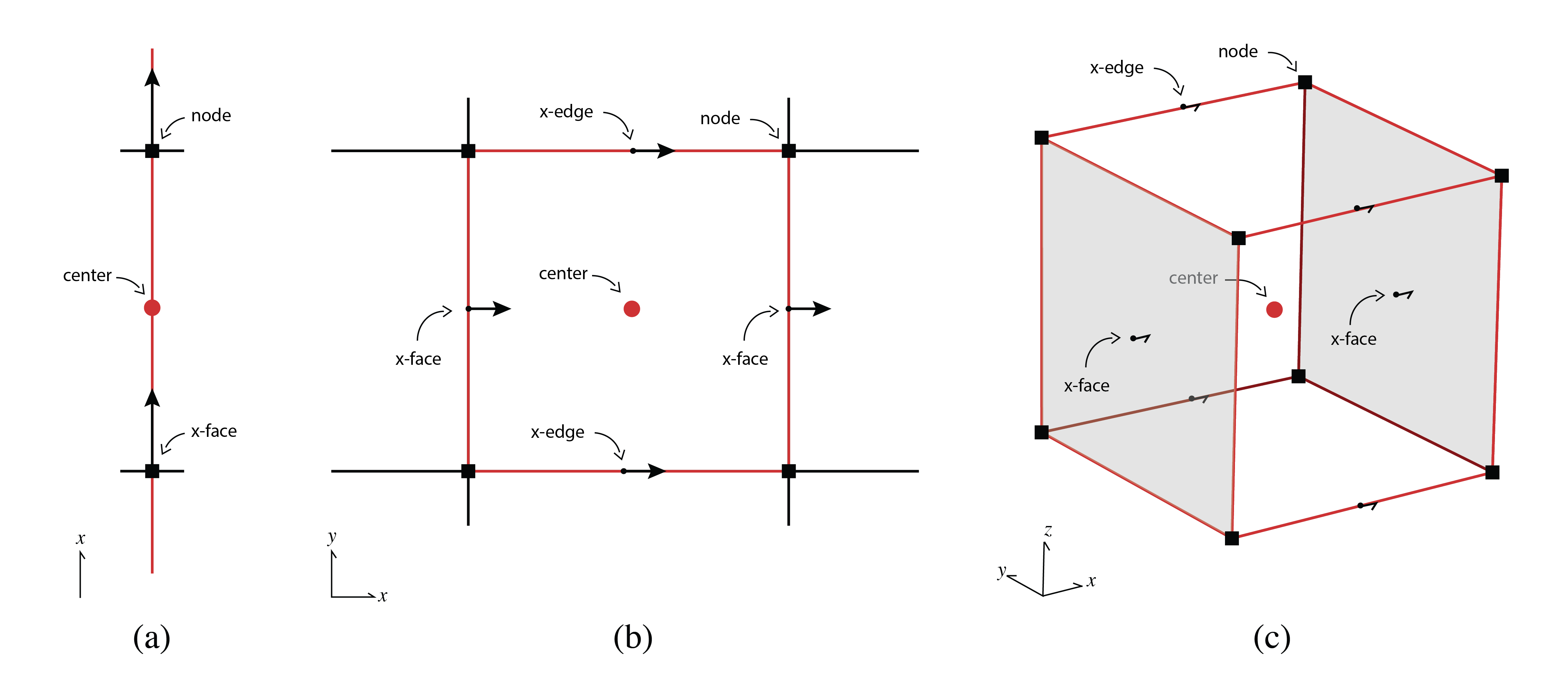
Figure B.2:Names of a finite volume cell on a tensor mesh in (a) one dimension, (b) two dimensions, and (c) three dimensions.
A cell face variable represents a vector that is a flux into or out of that face; the vector is pointed in the face normal direction, . As seen in the curvilinear cell in Figure B.3, the face normal directions may not be orthogonal, nor parallel to the Cartesian axes. However, as the direction of the face normal is a property of the mesh, the face variables only store the magnitude of the vector. A face variable on a single rectilinear cell is a length four array in 2D and a length six array in 3D. There are twelve edges in 3D, four in 2D, and one in 1D for each cell, all holding vector quantities that point in the tangent directions, . While cell faces represent fluxes, edges represent vector fields, as is the case in electromagnetics.
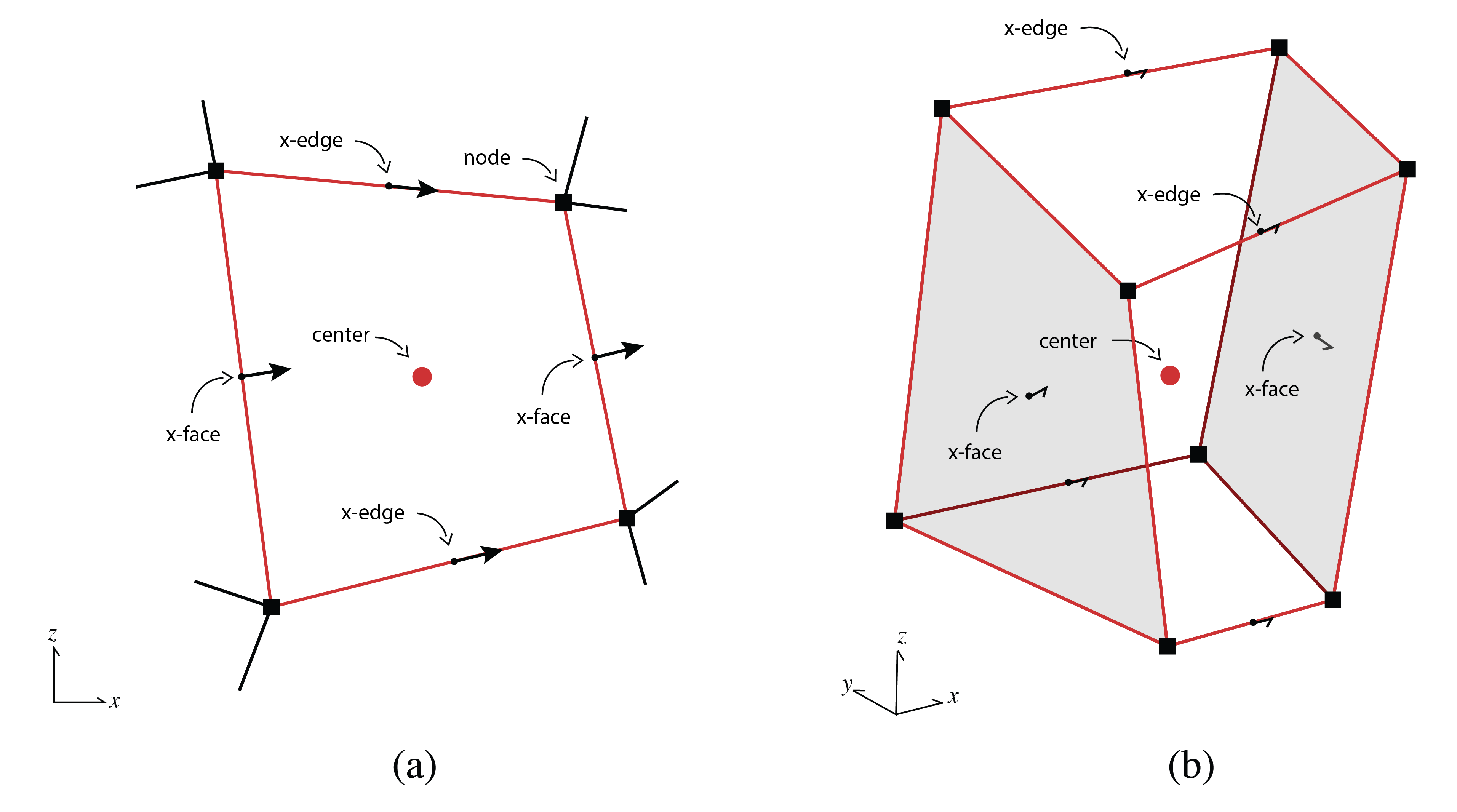
Figure B.3:Names of a finite volume cell on a curvilinear mesh in (a) two dimensions, and (b) three dimensions. Note that the cell faces and edges are no longer orthogonal.
Figure B.4 displays a tree mesh cell, which shows the location of hanging faces and nodes when two cells of different refinement levels share an interface. These hanging nodes, faces, and edges become important when computing the differential operators and inner products. A cylindrically symmetric mesh has the same structure as a tensor product mesh cell, except that all cells must be in the radial domain . It is tempting to conceptually locate the cell center of the first radial cell at , as this would be at the center of the cylinder. However, locating the cell center here violates our staggered grid in cylindrical coordinates and operators, such as the divergence, do not converge with second order accuracy. For consistency throughout the following sections, we will use terminology derived from a 3D cell. A cell's volume will refer to: volume in 3D; area in 2D; and length in 1D. Face areas will refer to the area perpendicular to a 3D face, which is a length in 2D and unity in 1D. Edge lengths will refer to lengths in 2D and will be in the same spatial locations as the cell faces (although with a different numbering and vector direction). In 1D, edge lengths will be the cell 'volumes' (lengths) and will be located at the cell centers. As such, the length of the 'volume' array will always be equal to the number of cells in the mesh.
B.2.3Numbering
The numbering of any mesh must be explicit in order to define arrays of properties, fields, and fluxes. The numbering of the mesh is arbitrary but has a number of consequences for the resulting differential operator matrices in terms of their structure and construction. In all logically rectangular meshes under consideration, we count first in the x, then y, then z dimensions. Counting in this way results in column vectorization and allows the use of Kronecker products for many of the matrix equations, specifically, the vectorization identity:
where is the discretized grid function, which is useful in building differential operators recursively from 1D operators. For non-logically rectangular meshes, such as quadtree and octree meshes, we sort the numbering first by distance along the x-axis, then y- and then z-. In the case of faces and edges where there are x-, y-, and z-components, we order these components separately and then concatenate them. The numbering is shown in Figure B.8a for a quadtree mesh for the cell centers, x-faces, and y-faces. Although Kronecker products can be used for logically rectangular meshes, this is not possible for tree-based meshes and the indexes must be kept track of 'by hand'.
It is important to know the number of variables for the discretization of grid variables. For a 3D logically rectangular mesh, the number of cells, nodes, faces, and edges are:
When comparing this to a cylindrically symmetric mesh, it is interesting to note that neither nodes nor faces exist, and edges only exist in the direction. A tree mesh has an added complication, which occurs when two adjacent cells have different refinement levels, leading to hanging nodes, edges, and faces. Figure B.4 schematically shows the locations of the hanging faces and nodes. When not dealt with, these complications cause numerical inaccuracies, which we will discuss further in Section B.3 on differential operators and Section B.4 on inner products.
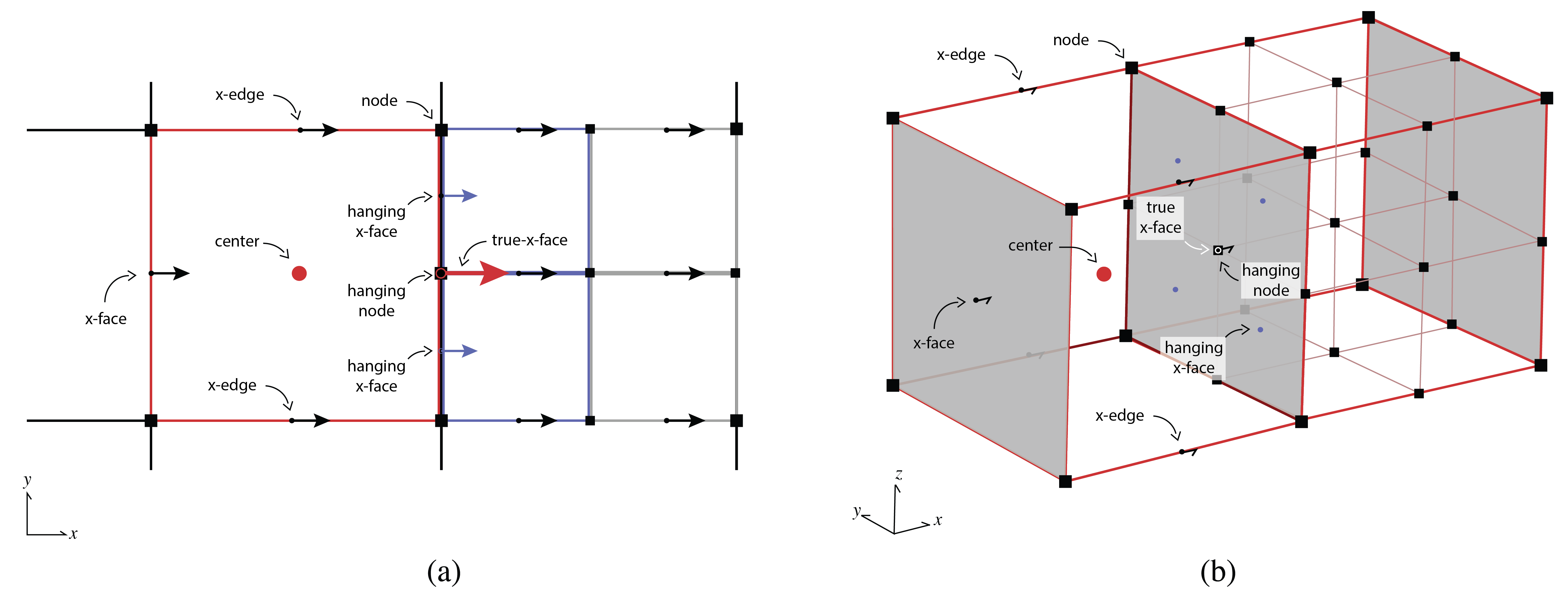
Figure B.4:Names of a finite volume cell on a tree mesh in (a) two dimensions, and (b) three dimensions. Note the location of hanging x-faces from the refined cells; hanging edges are not shown.
B.2.4DC resistivity equations
We will use the direct current (DC) resistivity problem from geophysics to motivate discretization of a parabolic partial differential equation and explain the various operators and operations necessary to consider for the finite volume technique. The equations for DC resistivity are derived in Figure B.5 and are further discussed in Pidlisecky et al., 2007. Conservation of charge (which can be derived by taking the divergence of Ampere’s law at steady state) connects the divergence of the current density everywhere in space to the source term, which consists of two point sources: one positive and one negative. The flow of current sets up electric fields according to Ohm’s law, which relates current density to electric fields through the electrical conductivity, . From Faraday’s law for steady state fields, we can describe the electric field in terms of a scalar potential, , which in a DC resistivity experiment is sampled at potential electrodes to obtain data in the form of potential differences. The first order form of the governing equations for DC resistivity are:
where is the input current at the positive and negative dipole locations, , captured as Dirac delta functions. To motivate the discretization of the DC resistivity equations, we will write the equations in weak form in the following section.
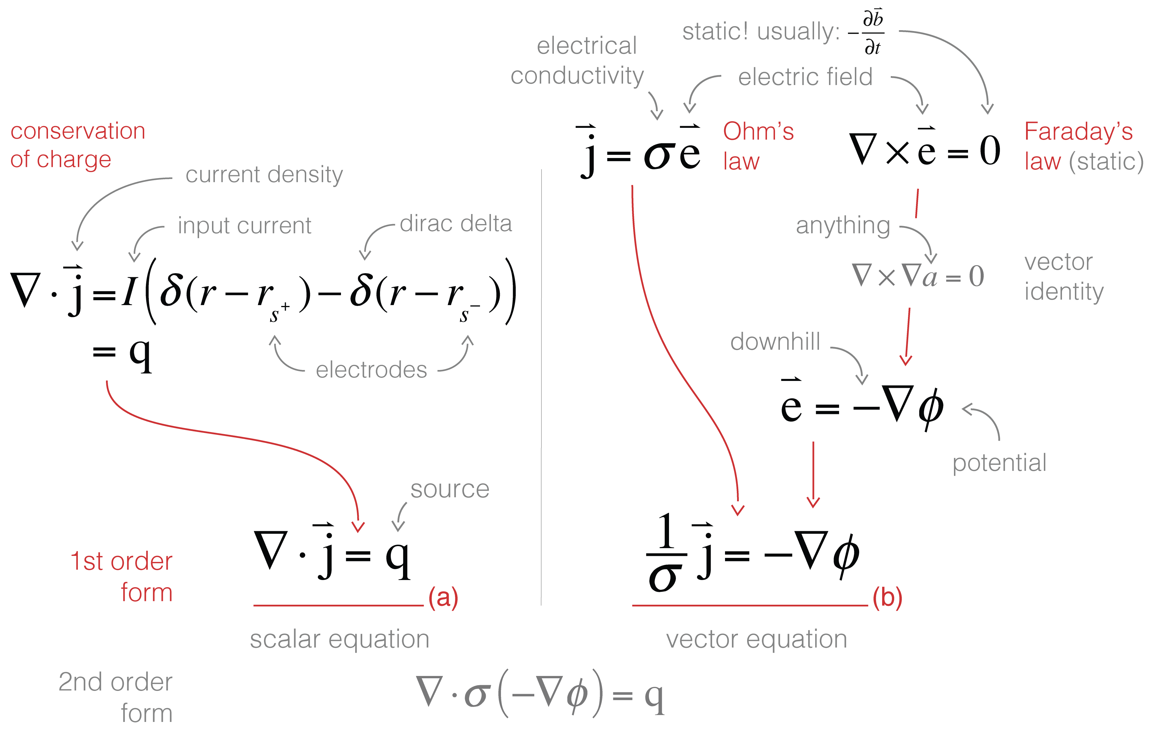
Figure B.5:Derivation of the direct current resistivity equations.
B.2.5Weak formulation
The weak formulation integrates the DC resistivity equations with a test function, , which reduces the requirement of differentiability (more details are available in Haber (2015)). To keep the notation clean, we also introduce notation , which we refer to as an inner product.
where the vectors and are arbitrary. The vector part of the DC resistivity equations (written in first order form) can be written in weak form as:
where is the test function. We can now employ a vector identity:
to integrate the right-hand side by parts. This integration results in the discretization of the DC resistivity equations entirely in terms of the divergence operator.
Here, if we assume Dirichlet boundary conditions for , that is, the potentials are zero far away from the domain of interest, we can use the divergence theorem to eliminate the second term on the right-hand side of the equation. This results in the following equation for DC resistivity with Dirichlet boundary conditions on :
We use Dirichlet for simplicity in this example. In practice, Neumann conditions are often used because 'infinity' needs to be further away, if applying Dirichlet boundary conditions, since potential falls off as and current density as .
Similar techniques for the weak formulation of Maxwell equations can be derived by applying the appropriate vector identities and boundary conditions. In the following two sections, we will discuss the differential operators and the discretization of inner products that are prevalent in the weak formulation.
B.3Operators
With the terminology and structure of the meshes well-defined, we can now create operators for the meshes. Although operators for averaging and interpolation are critical to any implementation, in this section, we will focus on the differential operators for the divergence, curl, and gradient. These operators take the form of sparse matrices, which are properties of each mesh. Although nuances exist in creating the operators for each mesh type, the basic building blocks come from the geometric concepts of individual cells, specifically the cell volume, face areas, and edge lengths. Given the cell spacings of tensor meshes, the computation of these properties is straightforward. For the cylindrical mesh, these values must be calculated in cylindrical coordinates. The volume and area calculations on the curvilinear mesh are straightforward in two dimensions. However, in three dimensions, the faces of the cell may not lie on a plane and, as a result, both the volume and face areas may not be well-defined. For face area, we use the average of the four parallelograms, which are calculated at each node of the face. As seen in Figure B.6, the cell volume is calculated by dividing the cell into five tetrahedrons and calculating the volume of each.

Figure B.6:Volume calculation using five tetrahedra.
B.3.1Divergence
The divergence is the integral of a flux through a closed surface as that enclosed volume shrinks to a point.
Since we have discretized and no longer have continuous functions, we cannot take the limit fully to a point. Instead, we approximate the limit around a finite volume: the cell. The flux out of the surface () is exactly how we discretized onto our mesh (i.e. ), except that the face normal points out of the cell (rather than in the coordinate directions). We can readily calculate the surface areas and normals of all cells in the mesh. The flux values on each cell face are discretized and represented by a scalar value pointing in the direction of the face normal. As such, we need only multiply these values by the face area and multiply by to ensure an outward facing normal with respect to the cell under consideration. To construct the divergence operator, , in one-dimension, the following discretization is used:
where is a sparse matrix with the cell volumes on the diagonal, is a 'stencil' matrix that ensures outward pointing normals, and is a diagonal matrix including the surface areas of each face. To move to higher dimensions, we exploit the logically rectangular structure and the column-ordered vectorization of the face variable. Kronecker products are used to place the difference matrix, , on the correct cells and faces. Not only is this conceptually efficient, when using an interpreted programming language, this also allows use of lower-level functions in compiled languages. For example, the divergence matrix in three-dimensions may be formed by:
where is the difference matrix in one-dimension for the th dimension. The is the identity matrix that has the length of the cells in the th dimension. Here the full divergence operator can be formed by:
The diagonal matrix, , contains the surface areas for each cell in the , , and directions, concatenated on the matrix diagonal. As the divergence only takes account of fluxes into and out of a cell in the direction of the face normal, this concatenation works for any logically rectangular mesh, regardless of orthogonality. For a cylindrical mesh, we need to give attention to the middle cylindrical cell where the flux at is known to be zero and, as such, this column can be removed from the matrix.

Figure B.7:Visual connection between the continuous and discrete representations of the divergence.
For a tree mesh, we need to pay special attention to the hanging faces to achieve second-order convergence for the divergence operator. Although the divergence cannot be constructed through Kronecker product operations, the initial steps are exactly the same for calculating the stencil, volumes, and areas. These steps yield a divergence defined for every cell in the mesh using all faces. However, redundant information exists when including hanging faces. As seen in Figure B.8, the x-face between the cells and cell 4 has three locations for an x-face variable, but there is conceptually only a single flux at that location: x-face 4. As such, we can construct a matrix that identifies these hanging faces and assigns them to the same face variable. This matrix includes only ones and can be multiplied on the right-hand side of the unreduced divergence. This ensures that the flux into the negative x-face of cell 4 in Figure B.8 has a single numeric value.
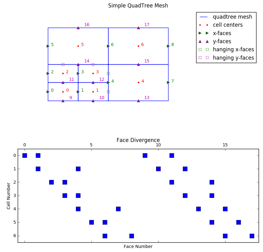
Figure B.8:Simple quadtree mesh showing (a) the mesh structure, cell numbering, and face numbering in both the and directions; and (b) the structure of the face divergence matrix that has eliminated the hanging faces.
B.3.2Curl
Similar to the divergence operator, we rely on the geometric interpretation of the curl:
where, is the outward facing normal, is the area of the face, and the line integral direction is oriented positively with respect to the normal (i.e. right-hand rule). Figure B.9 shows the integrating directions for a unit cube in each unit direction. To discretize the curl of an edge variable, we must integrate along each edge in the appropriate direction (i.e. multiply by ) and divide by the face area:
where is an edge length vector, and is the face area vector. The numeric curl on edges yields a vector variable on cell faces. Similar to the divergence operator, this definition can exploit the logically rectangular nature of the mesh and create the difference matrix, , using Kronecker products.

Figure B.9:Edge path integration or definition of the curl operator.
For the octree mesh, we need to treat both the hanging edges and faces to remove redundant information. Hanging edges are treated differently than faces. We can average the resulting flux from the curl operation through a face, from the five estimates of the flux to a single value over the larger face. We multiply this averaging matrix on the left-hand side of the unreduced curl matrix. The edges, however, need to be eliminated through linear interpolation of the coarse edges to the six refined edges in each direction on each coarse face. We multiply this interpolation on the right-hand side of the unreduced curl matrix. These two operations result in a curl that has eliminated both hanging edges and hanging faces through interpolation and averaging, respectively.
B.3.3Gradient
The gradient of a scalar function, , is a vector field whose dot product with an arbitrary vector, , yields the directional derivative in that direction.
In Cartesian coordinates (), this has the much more familiar form:
To discretize the gradient of a nodal variable, we can do a forward difference along all edges of the mesh and divide by the length of the edge tangents
where is the gradient stencil identifying the correct nodes, with , and is the lengths of the edges. Multiplying the gradient by some nodal variable, , results in a vector quantity that is the directional derivative along the edge tangent, which is a central difference and results in a variable located on the edges on the mesh. Alternatively, we can formulate the gradient for cell-centered, rather than nodal, variables. This formulation explicitly considers neighbouring cells, rather than just a single finite volume, and is a finite difference method. Although possible, this formulation is more cumbersome to represent on both tree meshes and curvilinear meshes or when anisotropy is considered. When a gradient is necessary in a differential equation, and the variable is located on cell centers instead of nodes, it is usually possible to rearrange the equations, using vector identities, to use the negative transpose of the divergence, as previously discussed.
For both the quadtree and octree meshes, we must once again deal with the hanging nodes and hanging edges. The treatment here is similar to that in the curl matrix. We interpolate hanging nodes from their neighbours (two in 2D, four in 3D) and the result of the gradient, an edge vector on all edges, is averaged to exclude the hanging edges.
Since we are using a staggered grid with centered differences, the discretization of the differential operators is second-order. That is, as we refine the mesh, our approximation of the divergence should improve by a factor of two. We can verify this numerical convergence using simple test functions with analytic expressions, well-chosen boundary conditions, and known derivatives. The assertion of this expectation of order is a critical piece of any numerical implementation.
B.4Inner products
Evaluating volume integrals over the cell becomes important when formulating equations in weak form, as in Section B.2.5. We can numerically evaluate these volume integrals in many different ways, however, the method must take into account the location and number of approximations of the integrand variables that are available. For two cell-centered variables, for example, the evaluation of the integral is simple and can be calculated by the midpoint approximation. The result is an inner product that includes a volume term, , for each cell:
Complications arise when we approximate the inner product but the variables do not live in the same location; that is, on the edges, faces, and cell centers.
B.4.1Face inner product
We use the face inner product when there is a multiplication between a cell-centered variable and a vector variable located on the faces. In the following example, we will use a cell-centered variable, , which is fully anisotropic, meaning that, in 3D, each cell is represented by a tensor. We multiply the tensor by and take the inner product with a face variable . When discretizing this integral, recall that the discretization has approximations, and , on each face of the cell. In 2D, that means two approximations of and two approximations of . In 3D, we also have two approximations of . Additionally, in the general case, these vectors may not be orthogonal nor axis aligned and so we must first transform them into their Cartesian components before multiplying by the discretized tensor, . Regardless of how we choose to approximate the vectors, and , we can represent this in vector form for every cell.
We multiply by square-root of volume on each side of the tensor, to keep symmetry in the system. Here, is an approximation of the Cartesian that must be calculated from known locations on the mesh, . There are many different ways to evaluate the inner product : we could approximate the integral using trapezoidal, midpoint, or higher order approximations, for example. A simple, second-order method is to break the integral into a sum of sections and apply the midpoint rule, where is the dimension of the mesh (i.e. two in 1D, four in 2D, and eight in 3D). For each of these sections, the midpoint rule uses the closest components of to compose a Cartesian vector. We use a matrix of size consisting of 0s and 1s, to select the appropriate faces to compose the corresponding vector .
Here, the index refers to the section where we choose to approximate this integral. In a curvilinear mesh, the fluxes chosen by are not necessarily axis-aligned and also may not be mutually orthogonal. As such, we must use a normalization to get back to Cartesian components, where multiplication with the is defined. These projection matrices, , are completed times for every cell of the mesh and, in 2D, have the form:
where is the normal to face . Solving for the Cartesian flux, , requires inverting a small matrix ( or ) for each section. We now have eight evaluations in 3D of the midpoint rule, using various approximations for . We can sum these approximations together to define the face inner product matrix, , for a logically rectangular mesh of any dimension, .
Here, each is a combination of the projection, volume, and any normalization to Cartesian coordinates. In a numerical implementation, it is often more efficient to complete this operation for each cell in the mesh at the same time, and return the sparse matrices for caching as this is a common operation in any inverse problem that estimates a cell-centered variable. For the tree mesh, we complete the face inner product identically as above, except for a final step to exclude the redundant hanging faces in the same way as the divergence matrix.
B.4.2Edge inner product
The edge inner product with a vector that is defined on the edges of a cell (rather than on the faces, as above) has a similar derivation. The difference comes in 3D, when selecting the edges around each node, as there are twelve edges instead of only six faces; these edges are selected by the matrix. Similarly, in the normalization to Cartesian coordinates, we use the edge tangent directions instead of using the face normals. The Cartesian edge values, , are projected using the tangents:
where is the projection matrix that selects the edges closest to each midpoint approximation. Once again, we compute the inner product by the mass matrix acting on the edges:
For the tree mesh, we complete the edge inner product as above, except with an added step to deal with the hanging edges. This step excludes the hanging edges through linear interpolation in the same way as the curl matrix.
B.4.3Tensor product mesh
The generality of this equation can be reduced when dealing with an axis-aligned tensor mesh with an isotropic physical property, . In this case, we do not need to take into account the normalization from . For a tensor mesh, the face inner product can be calculated as follows and can be interpreted as averaging the physical property between neighboring cells:
where is a Hadamard product for point-wise multiplication and is an averaging matrix from faces to cell centers. In one dimension this matrix has the form
The matrix has slight differences on a cylindrical tensor mesh to exclude the face. The 'averaging' matrix can be made for higher dimensions using Kronecker products and horizontal concatenation:
Note that this matrix is often referred to as the face-to-cell-center averaging matrix and, as such, is often divided by the dimension of the mesh to be a true average (i.e. there are three face averages above). If this is the case, care needs to be taken to restore this constant when calculating the inner product. Although general anisotropy is not easily added in this form, coordinate anisotropy can be added by composing this matrix as block diagonals instead of horizontal concatenation. Similarly, on a cylindrical mesh, if anisotropy is necessary, care should be taken that the anisotropy uses Cartesian, rather than cylindrical, coordinates, unless intended.
B.4.4Anisotropy
For defining isotropic, coordinate anisotropic, and fully anisotropic parameters, the following conventions are used in 3D:
In 2D, these conventions are similarly defined as:
Both the isotropic and coordinate anisotropic material properties result in a diagonal mass matrix on a tensor mesh. This is easy to invert if necessary. However, in the fully anisotropic case, or for any curvilinear mesh, the inner product matrix is not diagonal, as can be seen for a 3D mesh in the figure below.
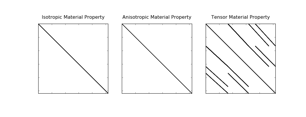
Figure B.10:Matrix structure of a face inner product of a cell centered physical property on a tensor mesh.
B.4.5Derivatives
In the context of parameter estimation, we are often interested in the parameters inside inner products and require efficient matrix-free derivatives for these elements. The derivative of these inner products is actually a tensor. However, the derivative is a matrix if we only require the computation of this product with a vector (as is usually the case). To show the computation of the inner product derivatives, we will consider a fully anisotropic tensor for a 3D logically rectangular mesh. Let us start with one part of the sum which makes up and take the derivative when this matrix is multiplied by some vector, :
Here, we will let and will have the form:
This matrix can subsequently be multiplied by . When multiplying these matrices by hand, we can see that they have the form:
where is the Hadamard product, and represents element-wise multiplication. We can now take the derivative with respect to any one of the parameters, for example,
Meanwhile, the derivative for is:
These derivatives are calculated for each of the eight components of the discretized inner product (four in 2D).
For a tensor product mesh with an isotropic physical property, this is again not the most efficient method of calculation. Instead, we can recall an alternative formula for calculating the inner product and take the derivative of that formula. We still must multiply by an arbitrary vector, :
Here, we calculate the derivative by exploiting the fact that a diagonal matrix and a vector can be multiplied in either order; that is, they are commutative.
The derivative, with respect to physical properties, becomes critical for the inverse problem, and is often not provided when implementations are solely focused on the forward simulation. In the implementation presented, we have given thought to accessing the derivatives of isotropic and anisotropic physical properties in an efficient way for all mesh types under consideration.
B.5Implementation
The discretize package (https://
B.5.1Organization
The object-oriented programming model in Python allows organization of the finite volume methods for the various meshes into a class inheritance structure. This organization has highlighted the similarities between techniques through elimination of redundant code between shared concepts and methods. Such elimination leads to a concise description of the differences between the methods, which was outlined in the previous section. We show our chosen organization in its entirety in Figure B.11. This figure shows the class inheritance and class properties of the discretize package and is best viewed in digital form.
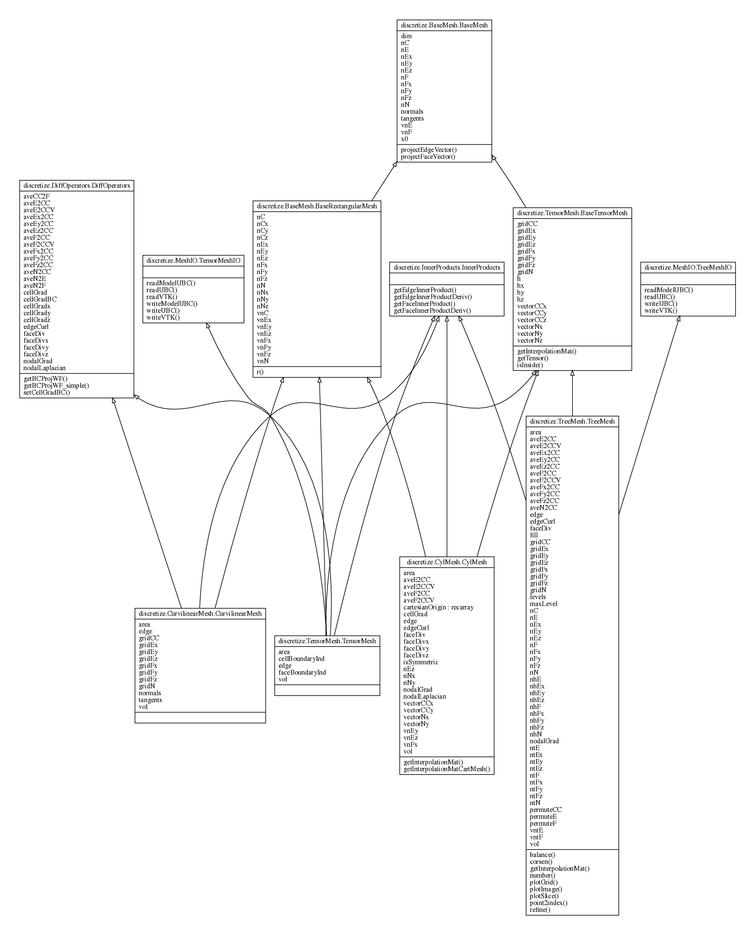
Figure B.11:The computational ontology developed for the discretize package showing inheritance and commonalities between the four mesh types.
There is a BaseMesh that has properties such as number of cells, nodes, faces, and edges nC, nN, nF and nE, respectively. We have decided to separate the differential, averaging and interpolation operators into their own class such that they can be included as a mixin (rather than inherited) into the final mesh classes. Methods for the inner products, IO to common formats, and visualization are also separated out and included as mixins. We have separated the concepts of being logically rectangular and being a tensor product mesh because these are different concepts. The basic counting of cells is on the rectangular mesh and the concept of a `cell-centered vector in the x dimension' is only for tensor product meshes. This inheritance demonstrates the concepts that: (a) the curvilinear mesh is rectangular, but not a tensor mesh; (b) the tree mesh is a tensor mesh, but not logically rectangular; and (c) the cylindrical mesh is both logically rectangular and a tensor mesh, however, through subtype polymorphism the cylindrical mesh overwrites the concepts for geometric calculations of volume, surface area, etc. as well as the counting for nodes, faces, and edges.
B.5.2User interface
Our goal for the implementation is to create a common programmatic terminology for working with finite volume techniques. By sharing the numerical implementation, not only is this 'language' precise, but it can also be tested for accuracy. A brief description of the implementation and use in practice, as well as a look at some of the major properties on the abstract mesh types in Table 2.1, was previously given in Section 2.3.4. As the implementation is openly available, we will point the reader to both the online, up-to-date documentation of each specific property and method (https://C, N, F, E to refer to cells, nodes, faces and edges, respectively. For example, for a tensor mesh the number of cells in the x-dimension would be called nCx, the nodal tensor of x-locations as a vector is called vectorNx, and the location of all face variables with an x-component is called gridFx. We named differential operators by the variable location that they act upon; for example: faceDiv and edgeCurl. These names allow us to define multiple operators. For example, the gradient can either operate on cell centers or nodes, cellGrad and nodalGrad, respectively. This language is common across all meshes considered and extends to other mesh types not yet implemented. As such, geophysical simulation codes can be built on top of this work to write PDEs in a declarative way, which is agnostic to the mesh implementation actually used. In collaboration with Heagy, Kang, Rosenkjaer and Mitchell simulations have been completed for time, frequency, and static implementations of electromagnetics using 1D, 2D, and 3D versions of the tensor, tree, curvilinear and cylindrically symmetric meshes Rosenkjaer et al., 2016Kang et al., 2015Heagy et al., 2015Heagy et al., 2014Cockett et al., 2014Kang et al., 2014Heagy et al., 2015Cockett & Haber, 2013Cockett et al., 2016Heagy et al., 2016Rosenkjaer et al., 2015Heagy et al., 2015. The terminology developed defines a clear interface, which allows for improvements in speed and functionality of the discretize package to transparently improve geophysical simulations.
The discretize interface allows for lazy loading of properties; that is, all properties of the mesh are created on demand and then stored for later use. This caching of properties is important, as not all operators are useful in all problems and, as such, are not created. The implementation here is different from some other finite volume implementations, as the operators are held in memory as matrices and are readily available for interrogation. We find this feature beneficial for educational and research purposes, as the discretization remains visually very close to the math, and the matrices can be manipulated, visually inspected, and readily combined.
The major difference between the mesh types is the instantiation of each type. A regular tensor mesh that is defined on the unit cube can be instantiated with integers. For example, TensorMesh([4, 8]) will create a 2D tensor mesh with equal spacings (a regular mesh) with nCx = 4 and nCy = 8 that has a domain over the unit square. Similarly, TensorMesh([hx, hy, hz]), where is a vector of variable cell spacings in the dimension, will create an irregularly spaced tensor mesh in 3D. To produce a cylindrically symmetric mesh (i.e. with a single cell in the azimuthal, , dimension), we can mix these notations. For example, CylMesh([hr, 1, hz]). For the definition of a CurvilinearMesh, all node locations must be specified in each dimension. These node locations may be provided as a list of either 2D or 3D matrices. For a tree mesh, a base mesh of tensor products are provided (which must be a power of 2), which represents the location of nodes at the lowest refinement level. A refinement function must also be provided. The refinement function is recursively passes cell centers and chooses whether that cell should be refined. This functional construction of the tree meshes encourages composable functions that refine based on, for example, location from a source and/or distance from a topographic interface. Alternatively, the mesh can be loaded from several formats (e.g. the UBC mesh and model files or the Open Mining Format (*.omf)). Once we have constructed the mesh, there is access to the differential operators, averaging and interpolation functions, and utilities for visualization and export.
B.6Numerical examples
Here we will briefly explore the application of the curvilinear mesh for a DC resistivity problem, which was introduced in Section B.2.4. We will explore the equations for a tensor mesh and a curvilinear mesh over a unit cube with Neumann boundary conditions. We tested the forward operators for analytical potential fields with the appropriate boundary conditions. A series of electrode arrays (surveys) were written to produce and collect data from the forward model. The survey used in this paper considered all receiver permutations in a grid on the top surface of the model. We note that it is not possible to experimentally collect data at the same location as the source electrodes; we discarded these permutations.
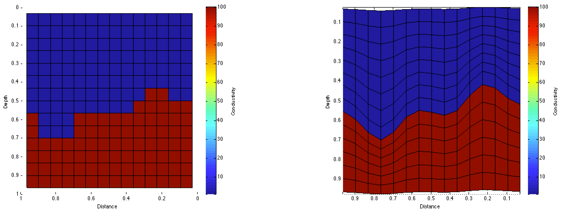
Figure B.12:Regular mesh and mesh aligned to layer for a simple conductivity model at .
For the numerical experiments presented here, we use a true model with a geologic interface with varying elevation. A cross-section through the 3D model at a mid-range discretization is seen in Figure B.12. The layer above the interface has a conductivity of 1 Sm and the layer below the interface has a conductivity of 100 Sm. We produced data from the forward operator, with the true model discretized, using cells. We created a series of models that ranged from to , over the same domain. At each discretization level, the true model was down-sampled onto a regular mesh as well as a curvilinear mesh that was aligned to the interface. The survey setup was a grid of equally spaced electrodes centered on the top surface of the model. There were a total of 16 electrodes, 120 source configurations, and 91 active measurements per source dipole. This gave rise to 10,920 total measurements, half of which are symmetric and likely would not have been collected in a field experiment, but were collected in this numerical experiment. We compare the data collected from each of the test models directly to the large model's data and plot the norm in Figure B.13. The mesh that is aligned to the layer performs significantly better at lower discretizations because it is more accurate at resolving the topographic interface. For example, at a norm data error of , the mesh aligned to the layer needed cells, versus when we used a rectangular discretization - or nearly five times the number of cells. The changes in error at coarse discretizations is due to the low accuracy in modeling the location of the sources and receivers.
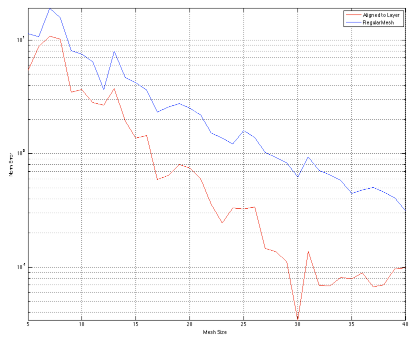
Figure B.13:Comparison of norm data error for the regular mesh and the mesh aligned to the interface.
The logically rectangular mesh allows increased degrees of freedom when placing the nodes of the mesh. In simple situations it is possible to significantly improve accuracy of the numerical model at reduced computational costs. However, the increased freedoms in picking node locations forces additional thought in mesh creation and alignment. Issues of mesh creation can be complex and these problems must be handled appropriately. It is suggested that simple meshes (i.e. regular) be used when possible and to only use the logically rectangular mesh when known layers, such as topography, are well-defined and known to significantly influence the solution of the problem and data collected.
B.7Conclusions
Discretization techniques are necessary in every aspect of computational geophysics and have been used extensively throughout my thesis and collaborative work. Many of the components in the discretization require special attention when considering the inverse problem; most notably, derivatives to the inner products and choosing when to cache operators. In this chapter, I have provided a description of the finite volume techniques that are necessary to discretize and simulate many of the elliptic and parabolic partial differential equations that are common in electromagnetic geophysics and hydrogeologic fluid flow. I have provided the derivations in a general form, such that they apply to four different types of meshes in common use in geophysical inverse problems. This generality allows for differences between the mesh types to be highlighted and discussed. I have also provided an open source, permissively licensed implementation of this work. The Python implementation, called discretize (https://
B.7.1Continuing work
A number of improvements and extensions that have yet to be tackled at the time of writing. Among these are (in no particular order): (a) improved ease of use around boundary conditions; (b) more utilities for mesh creation especially for more complicated meshes (i.e. curvilinear and tree); (c) an increase in the combinatorial nature of existing meshes, for example, cylindrical or curvilinear octrees; (d) extension to unstructured meshes, voronoi meshes, and other coordinate systems (e.g. spherical); (e) a more rigorous comparison to finite element codes (cf. Jahandari et al. (2017)); and (f) integration to existing mesh generation packages. By providing this package in an open, standalone, tested, documented form we hope that the implementation can be improved by the growing community of contributors.
- Doherty, J. (2004). PEST: Model independent parameter estimation. Fifth edition of user manual. Watermark Numerical Computing. 10.1016/B978-0-08-098288-5.00031-2
- Haber, E. (2015). Computational Methods in Geophysical Electromagnetics.
- Ascher, U. M., & Greif, C. (2011). A First Course in Numerical Methods. Society for Industrial. 10.1137/9780898719987
- Yee, K. S. (1966). Numerical solution of initial boundary value problems involving Maxwell’s equations in isotropic media. IEEE Trans. on Antennas and Propagation, 14, 302–307.
- Hyman, J. M., & Shashkov, M. (1999). Mimetic Discretizations for Maxwell’s Equations. 909, 881–909.