Simulation & Inversion Framework
2.1Introduction and motivation
Geophysical surveys can be used to obtain information about the subsurface, as the measured responses depend on the physical properties and contrasts in the earth. Inversions provide a mathematical framework for constructing physical property models consistent with the data collected by these surveys. The data collected are finite in number, while the physical property distribution of the earth is continuous. Thus, inverting for a physical property model from geophysical data is an ill-posed problem because no unique solution explains the data. Furthermore, the data may be contaminated with noise. Therefore, the goal of a deterministic inversion is not only to find a model consistent with the data, but also to find the 'best' model that is consistent with the data[1]. The definition of 'best' requires the incorporation of assumptions and a priori information, often in the form of an understanding of the particular geologic setting or structures Constable et al., 1987Oldenburg & Li, 2005Lelièvre et al., 2009. Solving the inverse problem involves many moving pieces that must work together, including physical simulations, optimization, linear algebra, and incorporation of geology. Deterministic geophysical inversions have been extensively studied and many components and methodologies have become standard practice. With increases in computational power and instrumentation quality, there is a greater drive to extract more information from geophysical data. Additionally, geophysical surveys are being applied in progressively more challenging environments. As a result, the geosciences are moving towards the integration of geological, geophysical, and hydrological information to better characterize the subsurface (e.g. Haber & Oldenburg (1997)Doetsch et al. (2010)Gao et al. (2012)). This integration is a scientifically and practically challenging task Li & Oldenburg, 2000Lelièvre et al., 2009. These challenges, compounded with inconsistencies between different data sets, often make the integration and implementation complicated and/or non-reproducible. The development of new methodologies to address these challenges will build upon, as well as augment, standard practices; this presupposes that researchers have access to consistent, well-tested tools that can be extended, adapted, and combined.
There are many proprietary codes available that focus on efficient algorithms and are optimized for a specific geophysical application (e.g. Kelbert et al. (2014)Li & Key (2007)Li & Oldenburg (1996)Li & Oldenburg (1998)). These packages are effective for their intended application; for example, in a domain-specific, large-scale geophysical inversion or a tailored industry workflow. However, many of these packages are 'black-box' algorithms; that is, they cannot easily be interrogated or extended. As researchers, we require the ability to interrogate and extend ideas; this must be afforded by the tools that we use. Accessibility and extensibility are the primary motivators for this work. Other disciplines have approached the development of these tools through open source initiatives, using interpreted languages such as Python (for example, Astropy in astronomy Astropy Collaboration et al., 2013 and SciPy in numerical computing Jones et al., 2001). Interpreted languages facilitate interactive development using scripting, visualization, testing, and interoperability with code in compiled languages and existing libraries. Furthermore, many open source initiatives have led to communities with hundreds of researchers contributing and collaborating by using social coding platforms, such as GitHub https://github.com. Initiatives also exist in the geophysical forward and inverse modeling community, which target specific geophysical applications (cf. Hansen et al. (2013)Hewett et al. (2013)Uieda et al. (2014)Kelbert et al. (2014)Harbaugh (2005)). Recent work has seen an increased focus by the geophysical community on a framework approach that targets multiple geophysical/hydrogeologic methods (e.g. JInv Ruthotto et al., 2016 and PyGIMLi Rücker et al., 2017). We are interested in creating a community around geophysical simulations and gradient-based inversions. To create a foundation on which to build a community, we require a comprehensive framework that is applicable across domains and upon which researchers can readily develop their own tools and methodologies. To support these goals, this framework must be modular and its implementation must be easily extensible by researchers.
2.1.1Attribution and dissemination
The goal of this chapter is to present a comprehensive framework for simulation and gradient-based parameter estimation in geophysics. Core ideas from a variety of geophysical inverse problems have been distilled to create this framework. We also provide an open source library, written in Python, called SimPEG (Simulation and Parameter Estimation in Geophysics, https://
To guide the discussion, we start this chapter by outlining gradient-based inversion methodology in Section 2.2. The inversion methodology directly motivates the construction of the SimPEG framework, terminology, and software implementation, which we discuss in Section 2.3. We weave an example of Direct Current (DC) resistivity throughout the discussion of the SimPEG framework to provide context for the choices made and highlight many of the features of SimPEG.
2.2Inversion methodology
Geophysical inverse problems are motivated by the desire to extract information about the earth from measured data. A typical geophysical datum can be written as:
where is a forward simulation operator that incorporates details of the relevant physical equations, sources, and survey design, is a generic symbol for the inversion model, is the noise that is often assumed to have known statistics, and is the observed datum. In a typical geophysical survey, we are provided with the data, , and some estimate of their uncertainties. The goal is to recover the model, , which is often a physical property. The data provide only a finite number of inaccurate constraints upon the sought model. Finding a model from the data alone is an ill-posed problem since no unique model exists that explains the data. Additional information must be included using prior information and assumptions (for example, downhole property logs, structural orientation information, or known interfaces Fullagar et al., 2008Li & Oldenburg, 2000Lelièvre et al., 2009). This prior knowledge is crucial if we are to obtain an appropriate representation of the earth and will be discussed in more detail in Section 2.2.1.
Defining and solving a well-posed inverse problem is a complex task that requires many interacting components. It helps to view this task as a workflow in which various elements are explicitly identified and integrated. Figure 2.1 outlines the inversion methodology that consists of inputs, implementation, and evaluation. The inputs are composed of: the geophysical data; the equations, which are a mathematical description of the governing physics; and, prior knowledge or assumptions about the setting. The implementation consists of two broad categories: the forward simulation and the inversion. The forward simulation is the means by which we solve the governing equations, given a model, and the inversion components evaluate and update this model. We are considering a gradient-based approach, which updates the model through an optimization routine. The output of this implementation is a model, which, prior to interpretation, must be evaluated. This requires considering, and often re-assessing, the choices and assumptions made in both the input and the implementation stages. In this chapter, our primary concern is the implementation component; that is, how the forward simulation and inversion are carried out numerically. As a prelude to discussing how the SimPEG software is implemented, we step through the elements in Figure 2.1, considering a Tikhonov-style inversion.
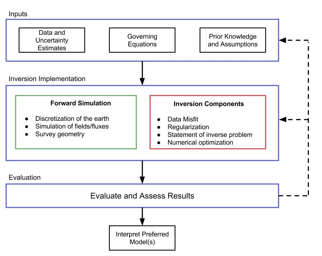
Figure 2.1:Inversion methodology. Including inputs, implementation, evaluation and interpretation.
2.2.1Inputs
Three sources of input are required prior to performing an inversion: (1) the geophysical data and uncertainty estimates; (2) the governing equations that connect the sought model with the observations; and (3) prior knowledge about the model and the context of the problem.
Data and uncertainty estimates
At the heart of the inversion are the geophysical data that consist of measurements over the earth. These data depend on the type of survey, the physical property distribution, and the type and location of the measurements. The details about the survey must also be known, such as the location, orientation, and waveform of a source and which component of a particular wavefield is measured at a receiver. The data are contaminated with additive noise, which can sometimes be estimated by taking multiple realizations of the data. However, standard deviations of those realizations only provide a lower bound for the noise. For the inverse problem, the uncertainty in the data must include not only this additive noise, but also any discrepancy between the true earth experiment and our mathematical representation of the data. Including these aspects requires accounting for mis-location of receivers and sources, poor control of the transmitter waveform, electronic gains or filtering applied to signals entering the receivers, incorrect dimensionality in our mathematical model (e.g. working in 2D instead of 3D), neglect of physics in our mathematical equations by introducing assumptions (e.g. using a straight ray tomography vs. a full waveform simulation in seismic), and discretization errors of our mathematical equations.
Governing equations
The governing equations provide the connection between the physical properties of the subsurface and the data we observe. Most frequently, these are sets of partial differential equations with specific boundary conditions. The governing equations, with specified source terms, can be solved through numerical discretization using finite volume, finite element, or integral equation techniques. Alternatively, they may also be solved through evaluations of analytic functions. Whichever approach is taken, it is crucial that there exists some way to simulate the data response given a model.
Prior knowledge
If one model acceptably fits the data, then infinitely many such models exist. Additional information is therefore required to reduce non-uniqueness. This additional information can be geologic information, petrophysical knowledge about the various rock types, borehole logs, additional geophysical data sets, or inversion results. This prior information can be used to construct reference models for the inversion and also characterize features of the model, such as whether it is best described by a smooth function or if it is discontinuous across interfaces. Physical property measurements can be used to assign upper and lower bounds for a physical property model at points in a volume or in various regions within our 3D volume. The various types of information relevant to the geologic and geophysical questions that we must address must be combined and translated into useful information for the inversion Lelièvre et al., 2009Li et al., 2010.
2.2.2Implementation
In this section, we outline the components necessary to formulate a well-posed inverse problem and solve it numerically. Two major abilities are critical to running the inversion: (1) the ability to simulate data, and (2) the ability to assess and update the model (Figure 2.1).
Forward simulation
The ability to carry out an inversion presupposes the ability to run a forward simulation and create predicted data, given a physical property model. In forward simulation, we wish to compute . The operator, , simulates the specific measurements taken in a geophysical survey, using the governing equations. The survey refers to all details regarding the field experiment that we need to simulate the data. The forward simulation of DC resistivity data requires knowledge of the topography, the resistivity of the earth, and the survey details, including locations of the current and potential electrodes, the source waveform, the units of the observations, and the polarity of data (since interchanging negative and positive electrodes may sometimes occur in the field). To complete the simulation, we need to solve our governing equations using the physical property model, , that is provided. In the DC resistivity experiment, our partial differential equation, with supplied boundary conditions, is solved with an appropriate numerical method; for example, finite volumes, finite elements, integral equations, or semi-analytic methods for 1D problems. In any case, we must discretize the earth onto an appropriate numerical forward simulation mesh, (). The size of the cells will depend upon the structure of the physical property model, topography, and the distance between sources and receivers. Cells in must be small enough, and the domain large enough, to achieve sufficient numerical accuracy. Proper mesh design is crucial so that numerical modeling errors are below a prescribed threshold value (cf. Haber (2015)).
In general, we can write our governing equations in the form of:
where is the modeled physical property and are the fields and/or fluxes. is often given by a partial differential equation or a set of partial differential equations. Information about the sources and appropriate boundary conditions are included in . This system is solved for and the predicted data are extracted from via a projection (or functional), . The ability to simulate the geophysical problem and generate predicted data is a crucial building block. Accuracy and efficiency are essential, since many forward problems must be evaluated when carrying out any inversion.
Inversion elements
In the inverse problem, we must first specify how we parameterize the earth model. Finding a distributed physical property can be done by discretizing the 3D earth into voxels, each of which has a constant, but unknown, value. It is convenient to refer to the domain on which this model is discretized as the inversion mesh, . The choice of discretization involves an assessment of the expected dimensionality of the earth model. If the physical property varies only with depth, then the cells in can be layers and a 1D inverse problem can be formulated. A more complex earth may require 2D or 3D discretizations. The choice of discretization depends on both the spatial distribution and resolution of the data and the expected complexity of the geologic setting. We note that the inversion mesh has different design criteria and constraints than the forward simulation mesh. For convenience, many inverse problems have historically been solved with = so that only one discretization is needed for the inversion. There is a growing body of work that investigates combinations of inversion discretizations and forward modeling meshes that are geared towards problem-specific formulations as well as efficiency in large-scale problems Haber & Schwarzbach, 2014Yang et al., 2014Haber & Heldmann, 2007. In any formulation, there exists a mapping between and such that the parameterization chosen can be used to simulate data in a forward simulation.
To formulate a mathematical statement of the inverse problem, there are two essential elements:
- data misfit: a metric that measures the misfit between the observed and predicted data; and
- regularization: a metric that is constructed to evaluate the model's agreement with assumptions and prior knowledge.
The data misfit requires an assessment of the error in each datum. These errors result from anything that yields a discrepancy between the mathematical modeling and the true value. It includes additive noise, errors in the description of survey parameters (e.g. receiver locations, transmitter waveforms, etc.), incorrect choice of governing equations, and numerical errors arising from the simulation technique. Clearly, quantifying the noise for each datum poses a challenge.
The data misfit is a measure of how well the data predicted by a given model reproduce the observed data. To assess goodness of fit, we select a norm that evaluates the 'size' of the misfit. This metric must include an uncertainty estimate for each datum. Often, we assume that the data errors are Gaussian and uncorrelated and then estimate the standard deviation for each datum. The most common norm, and one that is compatible with Gaussian statistics, has the form:
Here, is a forward modeling that produces predicted data, , as in equation: (2.1). is a diagonal matrix whose elements are equal to , where is an estimated standard deviation of the th datum. It is important to think carefully when assigning these estimates. A good option is to assign a . Percentages are generally required when there is a large dynamic range of the data. A percentage alone can cause great difficulty for the inversion if a particular datum acquires a value close to zero; therefore, we include a floor.
In addition to a metric that evaluates the size of the misfit, we also require a tolerance, . We consider that models satisfying adequately fit the data Parker, 1994. If the data errors are Gaussian and we have assigned the correct standard deviations, then the expected value of , where is the number of data. Finding a model that has a misfit substantially lower than this will result in a solution that has excessive and erroneous structure; that is, we are fitting the noise. Finding a model that has a misfit substantially larger than this will yield a model that is missing structure that could have been extracted from the data (see Oldenburg & Li (2005) for a tutorial).
The choice of misfit in equation (2.3) is not the only possibility for a misfit measure. If data errors are correlated, then is the square root of the data covariance matrix and it will have off-diagonal terms. Often useful in practice is recognizing if the noise statistics are non-Gaussian. Incorporating robust statistical measures, like norms with , are useful for handling outliers Ekblom, 1973Farquharson, 1998.
The second essential inversion element is defining the regularization functional. If there is one model that has a misfit equal to the desired tolerance, then there are infinitely many other models which can fit to the same degree. The challenge is to find the model that has both the desired characteristics and is compatible with a priori information. A single model can be selected from an infinite ensemble by measuring the length, or norm, of each model. Then the smallest, or sometimes largest, member can be isolated. Our goal is to design a norm that embodies our prior knowledge and, when minimized, yields a realistic candidate for the solution of our problem. The norm can penalize variation from a reference model, spatial derivatives of the model, or some combination of these. We denote this norm by and write it in a matrix form, for example,
is a matrix and is a reference model (which could be zero). The matrix can be a stacked combination of matrices weighted by :
Here, is a combination of smallness and first-order smoothness in the , , and directions. Each of the matrices is, in fact, a discrete representation of an integral (cf. Oldenburg & Li (2005)).
The final regularization, , can be a weighted sum of these, with being applied as scalars or diagonal matrices, with varying weights for each cell or cell face (cf. Oldenburg & Li (2005)Haber (2015)). Additional weightings can also be incorporated through , such as depth weighting, which is important in potential field inversions (such as magnetics and gravity), or sensitivity weightings to prevent model structure from concentrating close to sources or receivers Li & Oldenburg, 1996Li & Oldenburg, 2000. The regularization functionals addressed provide constraints on the model in a weak form; that is, a single number is used to characterize the entire model. Strong constraints that work within each cell can often be provided in the form of upper and lower bounds; these bounds will be incorporated in the following section. The norms referred to above are appropriate for many problems, however models norms, such as -norms, total variation, minimum support stabilizing functionals, or rotated smoothness operators that favor different character and/or include additional information can also be designed (cf. Oldenburg (1984)Oldenburg & Li (2005)Claerbout & Muir (1973)Strong & Chan (2003)Zhdanov (2002)Li & Oldenburg (2000)). For example:
The potential to have different norms tailored to a specific problem, with the additional functionality of localized weightings and reference models, provides the user with the capability of designing a regularization that favors a solution that is compatible with existing knowledge about the model. This task is not trivial, requires careful thought, and must often be re-evaluated and adjusted as the geophysicist iterates over the inversion procedure (Figure 2.1).
Statement of the inverse problem
The purpose of this section is to pose our inverse problem in a mathematically precise way and to provide a methodology by which a solution can be achieved. In the work that follows, we outline a specific methodology that we will later demonstrate. We formulate the inverse problem as a problem in optimization, where we define an objective function, based on the data misfit and model regularization, and aim to find a model which sufficiently minimizes it. Many variants of this formulation are possible.
At this stage of the workflow, we have on hand all of the necessary components for formulating the inverse problem as an optimization problem. We have the capability to forward model and generate predicted data, assess the data misfit using , and a tolerance on the data misfit has already been specified. A regularization functional, , and additional strong constraints on the model have been identified, such as upper and lower bounds: . The sought model is one that minimizes and also reduces the data misfit to some tolerance, . However, a reduction in data misfit requires that the model have increased structure, which typically is at odds with the assumptions we impose in the construction of , meaning that the and are antagonistic. To address this and still pose the inversion as an optimization problem, we design a composite objective function:
where is a positive constant. It is often referred to as the trade-off parameter, regression parameter, regularization parameter, or Tikhonov parameter Tikhonov & Arsenin, 1977. When is very large, the minimization of produces a model that minimizes the regularization term and yields a large . Alternatively, when is very small, minimization of produces a model that fits the data very well but is contaminated with excessive structure so that is large. The inverse problem is posed as:
Since the value of is not known a priori, the above optimization problem can be solved at many values of to produce a trade-off, or Tikhonov, curve (cf. Parker (1994)Hansen (1998)). An optimum value, , can be found so that minimizing equation (2.8) with produces a model with misfit . The value of can be found via cooling techniques where the is progressively reduced from some high value and the process stopped when the tolerance is reached or by using two-stage methods, as advocated by Parker (1977). There are other strategies for selecting the trade-off parameter including the L-curve technique Hansen, 1992, which attempts to find the point of greatest curvature in the Tikhonov curve and Generalized Cross Validation Wahba, 1990Golub et al., 1979Haber & Oldenburg, 2000Oldenburg & Li, 2005Farquharson & Oldenburg, 2004.
The optimization posed in equation (2.9) is almost always non-linear. It is linear only in a special case, where the forward mapping is a linear functional of the model, and are written as norms, is known, and there are no imposed bound constraints. This rarely happens in practice, requiring that iterative optimization methods be employed to find a solution. Gradient-based methods are commonly used and we refer the reader to Nocedal & Wright (1999) for background and introductions to the relevant literature. For geophysical problems, Gauss-Newton techniques have proven to be valuable and practical. For norms, we write the objective function as:
The gradient is given by:
where is the sensitivity or Jacobian. The components, , specify how the th datum changes with respect to the th model parameter; these changes will be discussed in more detail in the next section. At the th iteration, beginning with a model, , we search for a perturbation, , which reduces the objective function. Linearizing the forward simulation by:
and setting the gradient equal to zero yields the standard Gauss-Newton equations to be solved for the perturbation :
The updated model is given by:
where is a coefficient that can be found by a line search. Setting is the default and a line search is necessary if .
The iterative optimization process is continued until a suitable stopping criterion is reached. Completion of this iterative process yields a minimization for particular value of the trade-off parameter, . If we are invoking a cooling schedule, and if the desired misfit tolerance is not yet achieved, is reduced and the iterative numerical optimization procedure is repeated.
Sensitivities
A central element in the above approach is the computation of the sensitivities. The sensitivity functional is defined by:
where is a linear projection and indicates total difference. There are numerous approaches to computing the sensitivity, but the chosen methodologies are dictated by the size of the problem. The discrete sensitivity matrix, , is a dense matrix, where is the number of data and is the number of model parameters. For some problems, can be computed directly and stored. Ultimately, this computation and storage demands the solution of numerous forward problems (cf. Haber (2015)). In another approach, we can factor in symbolic form. In the general case, we solve for the sensitivity implicitly by taking the derivative of (equation (2.2)) to yield:
where indicates partial difference and both and are matrices. For a given model, corresponds to the forward simulation operator. If the forward problem is well-posed, then the matrix is invertible Haber, 2015. Equation (2.16) can be rearranged to:
and combined with equation (2.15) to obtain a formula for the sensitivity matrix. We note that this matrix is dense, often large, and need not actually be formed and stored.
Inversion as optimization
Once the inverse problem has been stated in an optimization framework (equation (2.9)), an appropriate optimization routine can be selected. For example, if bound constraints are incorporated, we can use a projected Gauss-Newton algorithm. In large-scale inversions, special attention may have to be given to ensuring a memory efficient optimization algorithm. However, the underlying mechanics of the algorithms often remain unchanged. In a geophysical inversion, we require a model that is consistent with a priori information and known, or assumed, statistical distributions (e.g. the discrepancy principle). As such, the stopping criteria of the inversion are often implemented differently than traditional optimization algorithms or a series of incomplete optimization algorithms are invoked while changing the objective function Oldenburg & Li, 2005Haber, 2015Haber et al., 2000.
The optimization of the stated inverse problem provides the machinery to obtain a mathematical solution. However, before the model is accepted as a viable candidate, there are numerous questions that should be investigated. For example, some questions to address might include: (a) How well does the recovered model fit the observed data? (b) Is there bias in the misfits between the observed and predicted data? (c) What was the path for the convergence? (d) Is there too much or too little structure? (e) Does the model fit with prior knowledge and other data sets? The final results and details about how the inversion algorithm has performed all provide clues as to whether the constructed model can be accepted or if elements in our procedure or its numerical implementation need to be altered and the inversion rerun. These might include: adjusting the assigned uncertainties in the misfit function; altering the model regularization; or, changing aspects of the numerical computations.
2.2.3Evaluation/interpretation
In this section, we return to the initial question posed, which the inversion was designed to help answer. Questions of interest might include: (a) Are the interesting features supported by the data or are they artifacts?; (b) Does the result make sense geologically and geophysically?; and (c) Are there interesting features that should be investigated further? Addressing these questions usually involves repeating the inversion process with appropriate modifications (cf. Oldenburg & Li (2005)Pidlisecky et al. (2011)Lines et al. (1988)). As such, we require an implementation that is inherently and unequivocally modular, with all pieces available for manipulation. Black-box software, where the implementations are hidden, obfuscated, or difficult to manipulate, does not promote experimentation and investigation. Exposing the details of the implementation to the geophysicist in a manner that promotes productivity and question-based interrogation is the goal of SimPEG and is the topic of the next section.
2.3Modular implementation
An overwhelming amount of choices must be made while working through the forward modeling and inversion process (Figure 2.1). As a result, software implementations of this workflow often become complex and highly interdependent, making it difficult to interact with other scientists or to ask them to pick up and change the work. Our approach to handling this complexity is to propose a framework, Figure 2.2, which compartmentalizes the implementation of inversions into various units. We present the framework in this specific modular style, as each unit contains a targeted subset of choices crucial to the inversion process. The aim of the SimPEG framework, and implementation, is to allow users to move between terminology, math, documentation, and code with ease, such that there is potential for development in a scalable way. The SimPEG implementation provides a library that mimics the framework shown in Figure 2.2, with each unit representing a base class. These base classes can be inherited in specific geophysical problems to accelerate development as well as to create code that is consistent between geophysical applications.
2.3.1Implementation choices
We chose Python Van Rossum & Drake Jr, 1995 for the implementation of SimPEG. Python supports object-oriented practices and interactive coding, has extensive support for documentation, and has a large and growing open source scientific community Lin, 2012. As an interpreted language, however, there are occasionally bottlenecks on speed or memory. These inefficiencies may mean that the code will not be able to scale to a production quality code. However, these computational bottlenecks can often be identified through profiling and can be written in a lower-level language and wrapped in Python. Additionally, these problems are admissible when the goal of the software is clear: we require an interactive research tool where geophysical problems from many disciplines live in one place to enhance experimentation and dissemination of new ideas. To enhance the dissemination of our work, we have released our work under the permissive MIT license for open source software. The MIT license neither forces packages that use SimPEG to be open source, nor does it restrict commercial use. We have also ensured that we have followed best practices, with regard to version control, code-testing, and documentation Wilson et al., 2014.
2.3.2Overview
As discussed in the previous section, the process of obtaining an acceptable model from an inversion generally requires the geophysicist to perform several iterations of the inversion workflow while rethinking and redesigning each piece of the framework to ensure it is appropriate in the current context. Inversions are experimental and empirical by nature and our software package is designed to facilitate this iterative process. To accomplish this iterative process, we have divided the inversion methodology into eight major components (Figure 2.2). The Mesh class handles the discretization of the earth and also provides numerical operators. The forward simulation is split into two classes: the Survey and the Problem. The Survey class handles the geometry of a geophysical problem as well as sources. The Problem class handles the simulation of the physics for the geophysical problem of interest. Although created independently, these two classes must be paired to form all of the components necessary for a geophysical forward simulation and calculation of the sensitivity. The Problem creates geophysical fields, given a source from the Survey. The Survey interpolates these fields to the receiver locations and converts them to the appropriate data type (for example, by selecting only the measured components of the field). Each of these operations may have associated derivatives, with respect to the model and the computed field; these associated derivatives are included in the calculation of the sensitivity. For the inversion, a DataMisfit is chosen to capture the goodness of fit of the predicted data and a Regularization is chosen to handle non-uniqueness. These inversion elements and an Optimization routine are combined into an inverse problem class (InvProblem). InvProblemis the mathematical statement (i.e. similar to equation (2.9)) that will be numerically solved by running anInversion. The Inversion class handles organization and dispatch of directives between all of the various pieces of the framework.

Figure 2.2:SimPEG framework indicating the flow of information. In the implementation, each of these modules is a base class.
The arrows in Figure 2.2 indicate what each class takes as a primary argument. For example, both the Problem and Regularization classes take a Mesh class as an argument. The diagram does not show class inheritance, as each of the base classes outlined have many subtypes that can be interchanged. The Mesh class, for example, could be a regular Cartesian mesh or a cylindrical coordinate mesh, which have many common properties. We can exploit these common features, such as both meshes being created from tensor products, through inheritance of base classes; differences can be expressed through subtype polymorphism. We refer the reader to the online, up-to-date documentation (https://
2.3.3Motivating example
We will use the DC resistivity problem from geophysics to motivate and explain the various components of the SimPEG framework. This example will be referred to throughout this section. We will introduce the example briefly here and refer the reader to Appendix \ref{sec:dc-derivation} for a more in-depth discussion. The governing equations for DC resistivity are:
where is the electrical conductivity, is the electric potential, and is the input current at the positive and negative dipole locations , captured as Dirac delta functions. In DC resistivity surveys, differences in the potential field, , are sampled using dipole receivers to collect observed data. To simulate this partial differential equation (PDE) (or set of PDEs, if there are multiple current injection locations), we must discretize the equation onto a computational mesh.
2.3.4Mesh
Any numerical implementation requires the discretization of continuous functions into discrete approximations. These approximations are typically organized in a mesh, which defines boundaries, locations, and connectivity. In geophysical simulations, we require the definitions of averaging, interpolation, and differential operators for any mesh. Throughout our work, we have implemented discretization techniques, using a staggered mimetic finite volume approach Hyman & Shashkov, 1999Hyman et al., 2002. For an in-depth discussion of the finite volume techniques employed in this thesis, we refer the reader to Appendix \ref{ch:discretize}. This work has resulted in an open source package called discretize, which provides finite volume techniques abstracted across four mesh types: (1) tensor product mesh; (2) cylindrically symmetric mesh; (3) logically rectangular, non-orthogonal mesh; and (4) octree and quadtree meshes. The techniques and interface to the methodologies are specifically tailored for efficiency and accessibility for geophysical inverse problems. To create a new Mesh instance, a TensorMesh class can be selected from the discretize module and instantiated with a list of vectors:
import discretize  # See Appendix A and Cockett et al. 2016
import numpy as np
import scipy.sparse as sp
hx = np.ones(30)
hy = np.ones(30)
mesh = discretize.TensorMesh([hx, hy])
Creation of a 2D tensor product mesh using the discretize package discussed in Appendix \ref{ch:discretize}.
Here, we import the discretize library as well as NumPy (np) and SciPy's sparse matrix package (sp) Oliphant, 2007Jones et al., 2001. The vectors hx and hy describe the cell size in each mesh dimension. The dimension of the mesh is defined by the length of the list, requiring very little change to switch mesh dimensions or type. Once an instance of a mesh is created, access to the properties and methods, shown in Table 2.1, is possible. Additional methods and visualization routines are also included in the Mesh classes. Of note in Table 2.1 are organizational properties (such as counting and geometric properties), locations of mesh variables as Cartesian grids, differential and averaging operators, and interpolation matrices. We can readily extend the mesh implementation to other types of finite volume meshes (for example, octree Haber & Heldmann, 2007, logically rectangular non-orthogonal meshes Hyman et al., 2002, and unstructured meshes Ollivier-Gooch & Van Altena, 2002). Additionally, this piece of the framework may be replaced by other methodologies such as finite elements.
Table 2.1:Selected Mesh class properties with explanations.
| Property or Function | Explanation |
|---|---|
dim | Dimension of the mesh |
x0 | Location of the origin |
nC, nN, nF, nE | The number of cells, nodes, faces, or edges. (e.g. nC is the total number of cells) |
vnC, vnN, vnF, vnE | Number of cells as vectors (e.g. vnC == [nCx, nCy, nCz]) |
vol, area, edge | Geometric measurements for the mesh (w.r.t. 3D nomenclature) |
gridN, gridCC, etc. | Array of grid locations |
nodalGrad | Gradient of a nodal variable edge variable |
faceDiv | Divergence of a face variable cell-centered variable |
edgeCurl | Curl of a edge variable face variable |
cellGrad | Gradient of a cell-centered variable face variable |
aveF2CC, aveN2CC, etc. | Averaging operators (e.g. FCC, takes values on faces and averages them to cell-centers) |
getInterpolationMat(loc) | Interpolation matrix for xyz locations |
With the differential operators readily accessible across multiple mesh types, simulation of a cell-centered discretization for conductivity, , in the DC resistivity problem is straightforward. The discretized system of equations, (2.18), can be written as:
where and are the divergence and 'gradient' operators, respectively. This equation is assuming Dirichlet boundary conditions and a weak formulation of the DC resistivity equations, as in Section B.2.5. The conductivity, , is harmonically averaged from cell-centers to cell-faces to create the matrix Pidlisecky et al., 2007. Using our discretize package, this equation is written as:
D = mesh.faceDiv
Msig = mesh.getFaceInnerProduct(sigma, invProp=True, invMat=True)
A = D*Msig*D.T
Creation of the matrix for the direct current resistivity problem. See Appendix \ref{ch:discretize} for details on finite volume.
The code is easy to read, looks similar to the math, can be built interactively using tools such as IPython Pérez & Granger, 2007, and is not dependent on the dimension of mesh used. Additionally, it is decoupled from the mesh type. For example, Figure 2.3 is generated by solving a DCProblem for three different mesh types: TensorMesh; TreeMesh; and, CurvilinearMesh. Other than the specific mesh generation code, no other modifications to the DC problem were necessary (see the online examples provided in SimPEG). Given the electrode locations, a can be constructed on each mesh and the system, , can be solved.
There are many excellent packages available to solve matrix equations and we have created a library to interface many of these direct and iterative solvers. The package, pymatsolver, comes with a few different types of Solver objects that provide a simple and common interface to Super-LU, Paradiso, and Mumps as well as including a few simple preconditioners for iterative solvers, Li (2005)Schenk & G̈artner (2004)Duff et al. (1986)Balay et al. (2012).
from pymatsolver import PardisoSolver  # Solver wrapping utilities
Ainv = PardisoSolver(A)  # Create a solver object
u = Ainv * (- q)
mesh.plotImage(u)
Solving and plotting the fields () for direct current resistivity using pymatsolver and visualization utilities in SimPEG.
The potential field can be projected onto the receiver electrode locations through interpolation matrices, which are constructed by the Mesh class. Additionally, there are multiple visualization routines that have been included in the Mesh class for rapid visualization and interrogation of geophysical fields and physical properties (Figure 2.3). We note that these code snippets can be easily be combined in a script, highlighting the versatility and accessibility of the Mesh classes in discretize.

Figure 2.3:Solving the DC resistivity problem for a dipole and using the meshes visualization routine for the potential, , for three different mesh types: (a) TensorMesh, (b) TreeMesh, and (c) CurvilinearMesh. The potential has been interpolated onto the tensor mesh for visualization.
This script will be expanded upon and segmented into the various pieces of the framework in the following sections. We find that the development of geophysical codes is often iterative and requires 'scripting' of equations. Only after these equations are correct, as demonstrated by an appropriate test (e.g. Tests.checkDerivative), do we formalize and segment our script to enable a geophysical inversion to be run. The toolbox that SimPEG provides promotes this interactive and iterative style of development.
2.3.5Forward simulation
The forward simulation in SimPEG is broken up into a Survey class and a Problem class. The Problem class contains the information and code that capture both the physics used to describe the connection between a physical property distribution and the fields/fluxes that are measured in a geophysical survey. The Survey class contains information about the observed data and the geometry of how to collect the data (e.g. locations and types of receivers and sources) given a Problem that simulates fields. The Problem and the Survey must be paired together to simulate predicted data. We decided on this separation of the code because it is possible to have multiple mathematical descriptions, of varying complexities, which explain the same observed data. For example, a seismic simulation could have multiple approximations to the physics, which increase in complexity and accuracy, from straight-ray tomography or Eikonal tomography to full waveform simulation. Additionally, there are often multiple types of geophysical surveys that could be simulated from the same Problem class.
Table 2.2:Base Problem class properties with explanations.
| Property or Function | Explanation |
|---|---|
fields(m) | Calculation of the fields given a model |
Jvec(m, v) | Sensitivity times a vector |
Jtvec(m, v) | Adjoint sensitivity times a vector |
Jfull(m) | Full sensitivity matrix |
mapping | Maps the model to a physical property |
The crucial aspects of the Problem class are shown in Table 2.2 and the properties and methods of the Survey class are shown in Table 2.3. We note that each of the sub-classes of Problem will implement fields and sensitivities in a different way, likely with additional methods and properties. Furthermore, the choice of terminology becomes clearer when these classes are inherited and used in a specific geophysical method (e.g. a DCProblem or EMProblem). For the DCProblem, the fields can be created by constructing and solving with the source terms, , which will be provided by the DCSurvey's source list (srcList). Each source has at least one receiver associated with it and the receivers can create a matrix, , which project the fields, , onto the data-space. For example, in the DC problem, a dipole receiver samples the potential at each electrode location and computes the difference to give a datum. We note that the process of computing a datum may be more involved and have derivatives with respect the computed fields and, possibly, the model. We solve much of the organizational bottlenecks through general receiver and source classes, which can be inherited and tailored to the specific application. The mapping in the Problem provides a transformation from an arbitrary model to a discretized grid function of physical properties. For example, log-conductivity is often used in the inverse problem for DC resistivity, rather than parameterizing directly in terms of conductivity. If this choice is made for the model, an appropriate map (i.e. the exponential) must be provided to transform from the model space to the physical property space (cf. Heagy et al. (2014)).
Table 2.3:Selected Survey class properties with explanations.
| Property or Function | Explanation |
|---|---|
dobs, nD | , number of data |
std | Estimated standard deviations |
srcList | List of sources with associated receivers |
dpred(m) | Predicted data given a model, |
projectFields(m, u) | Projects the fields, |
projectFieldsDeriv(m, u) | Derivative of the projection, |
residual(m) |
2.3.6DC resistivity forward simulation
We present a simple DC-resistivity survey to demonstrate some of the components of SimPEG in action. We use a set of Schlumberger arrays to complete a vertical sounding. In this example, we have taken our scripts from the previous section describing the forward simulation and combined them in a package called simpegDC (https://simpeg.xyz). We use the 3D tensor mesh to run the forward simulation for the data of this problem.
from SimPEG.EM.Static import DC
survey = DC.SurveyDC(srcList)
problem = DC.ProblemDC(mesh)
problem.pair(survey)
data = survey.dpred(sigma)
Pairing the Problem and Survey objects to create predicted data, .
Here the srcList is a list of dipole sources (DC.SrcDipole), each of which contains a single receiver, (DC.RxDipole). Similar to the illustration in Figure 2.2, the Problem and the Survey must be paired for either to be used to simulate fields and/or data. These elements represent the major pieces of any forward simulation in geophysics; they are crucial and must be well-tested for accuracy and efficiency before any attempt is made at setting up the inverse problem.
2.3.7Sensitivities
The sensitivity and adjoint will be used in the optimization routine of the inversion. Inefficient or inaccurate calculation of the sensitivities can lead to an extremely slow inversion. This is critical in large-scale inversions, where the dense sensitivity matrix may be too large to hold in memory directly. As discussed in the methodology section, the sensitivity matrix need not be explicitly created when using an iterative optimization algorithm, such as Gauss-Newton ((2.13)), solved with a conjugate gradient approach. The calculation of vector products with the sensitivity matrices is an important aspect of SimPEG, which has many tools to make construction and testing of these matrices modular and simple. For the DC resistivity example, the discretized governing equations are written as: . We can implement the sensitivity equations (2.15) and (2.17) to yield:
where is a known sparse matrix, is the forward operator and is equivalent to , and is a projection matrix (cf. Pidlisecky et al. (2007)). Each matrix in this expression is sparse and can be explicitly formed; however, the product is dense and holding it in memory may not be possible. If an iterative solver is used in the optimization, only matrix vector products are necessary and the sensitivity need not be explicitly calculated or stored. Program 2.5 outlines the calculation of Jvec, given a model, m, the fields, u, and a vector to multiply, v. In Program 2.5, we draw the distinction between the model, m, and the conductivity, sig, which are connected through a mapping, , and associated derivatives. The matrix, , is denoted dCdm and formed by looping over each source in the DC resistivity survey.
def Jvec(self, m, v, u=None):
    # Set current model; clear dependent property $\mathbf{A(m)}$
    self.curModel = m
    sigma = self.curModel.transform # $\sigma = \mathcal{M}(\mathbf{m})$
    if u is None:
        # Run forward simulation if $u$ not provided
        u = self.fields(self.curModel)
    else:
        shp = (self.mesh.nC, self.survey.nTx)
        u = u.reshape(shp, order='F')

    D = self.mesh.faceDiv
    G = self.mesh.cellGrad
    # Derivative of model transform, $\frac{\partial \sigma}{\partial \mathbf{m}}$
    dsigdm_x_v = self.curModel.transformDeriv * v

    # Take derivative of $C(\mathbf{m}, \bfu)$ w.r.t. $\mathbf{m}$
    dCdm_x_v = np.empty_like(u)
    # loop over fields for each transmitter
    for i in range(self.survey.nTx):
        # Derivative of inner product, $\left(\mathbf{M}_{1/\sigma}^f\right)^{-1}$
        dAdsig         = D * self.dMdsig( G * u[:,i] )
        dCdm_x_v[:, i] = dAdsig *  dsigdm_x_v

    # Take derivative of $C(\mathbf{m}, \bfu)$ w.r.t. $\bfu$
    dCdu = self.A
    # Solve for $\frac{\partial \bfu}{\partial \mathbf{m}}$
    dCdu_inv = self.Solver(dCdu, **self.solverOpts)
    P        = self.survey.getP(self.mesh)
    J_x_v    = - P * mkvc( dCdu_inv * dCdm_x_v )
    return J_x_v
Program 2.5:Sensitivity times a vector method for the DCProblem.
2.3.8Inversion elements
As indicated in the methodology section, there are two key elements needed for a geophysical inversion: DataMisfit and Regularization. The DataMisfit must have a way to calculate predicted data and, as such, it takes a paired survey as an initial argument, which allows forward simulations to be completed. DataMisfit and Regularization have similar interfaces, which are shown in Table 2.4. The DataMisfit class also has a property, targetMisfit, for the target misfit, which can be checked by an InversionDirective and used as a stopping criteria. As discussed in the methodology section, the Regularization is defined independently from the forward simulation. The regularization is with respect to the model, which may or may not be on the same mesh as the forward simulation (i.e. ). In this case, a mapping of a model to a physical property on the forward simulation mesh is necessary for the Problem. The Regularization class also has a mapping property, which allows a wide variety of regularizations to be implemented (e.g. an active cell map used to ignore air cells). As such, the Regularization mapping is often independent from the mapping in the Problem class, which outputs a physical property. Included in the SimPEG package are basic Tikhonov regularization routines and simple norms for both Regularization and DataMisfit classes. Each of these classes has properties for the appropriate model and data weightings, as discussed in the previous section (e.g. and ). These classes are readily extensible, such that they can be customized to specific problems and applications (for example, considering or norms or customized regularizations).
Table 2.4:Common functions for the Regularization, and DataMisfit classes.
| Function | Explanation |
|---|---|
obj(m) | Evaluate the functional given a model when the class is called directly. |
obj.deriv(m) | First derivative returns a vector. |
obj.deriv2(m, v) | Second derivative as an implicit operator. |
2.3.9Inverse problem and optimization
The InvProblem combines the DataMisfit and Regularization classes by introducing a trade-off parameter, . In addition to the trade-off parameter, there are methods that evaluate the objective function and its derivatives (Table 2.4). Additional methods can save fields so that information is not lost between evaluation of the objective function and the derivatives. The InvProblem may also include bounds on the model properties so that they can be used in the optimization routine. If we consider a joint or integrated inversion, multiple data misfit functions, employing different physics, and that multiple types of regularization functionals may be summed together, possibly with relative weightings, we can define the InvProblem (cf. Lines et al. (1988)Holtham & Oldenburg (2010)Heagy et al. (2014)). Once the InvProblem can be evaluated to a scalar with associated derivatives, an Optimization can either be chosen among the ones included in SimPEG or provided by an external package. Optimization routines in SimPEG include steepest descent, L-BFGS, and Inexact Gauss-Newton (cf. Nocedal & Wright (1999)). The components are relatively simple to hook up to external optimization packages (for example, with the optimization package in SciPy Jones et al., 2001).
2.3.10Inversion
The Inversion conducts all communication between the various components of the framework and is instantiated with an InvProblem object. The Inversion has very few external methods but contains the list of directives that are executed throughout the inversion. Each InversionDirective has access to the components of the inversion framework and can thus access and change any of these components while the inversion is running. A simple directive may print optimization progress or save models to a database. More complicated directives may change or compute parameters such as, , reference models, data weights, or model weights. These directives are often guided by heuristics, but versions can often be formalized (see, for example, the iterative Tikhonov style inversion Tikhonov & Arsenin, 1977Parker, 1994Oldenburg & Li, 2005). There are many computational shortcuts that may be investigated, such as how many inner and outer CG iterations to complete in the inexact Gauss-Newton optimization and whether the number of iterations should change as the algorithm converges to the optimal model. The directiveList in the Inversion encourages heuristics, which geophysicists often complete 'by hand', to be codified, combined, and shared via a plug-in style framework.
2.3.11DC resistivity inversion
We will build on the example presented in Section 2.3.6, which has a survey setup that only provides enough information for a vertical sounding. As such, we will decouple our 3D forward mesh and 1D inversion mesh and connect them through a mapping (cf. Kang et al. (2015)). Additionally, since electrical conductivity is a log-varying parameter, we will also construct a model space that is optimized in log space. Both of these model transformations will be handled with a single map, , where .
from SimPEG import Maps
mapping = Maps.ExpMap(mesh) * Maps.SurjectVertical1D(mesh)
sigma = mapping * model
Creation and chaining together of multiple mapping properties for a model of .
We have provided a number of common mapping transformations in the SimPEG.Maps package and these can be easily combined with a multiplication symbol. Additionally, when using these maps, we calculate the derivatives using the chain rule, allowing them to be easily included in the sensitivity calculation (cf. Program 2.5, line 15). Figure 2.4 demonstrates this mapping visually.

Figure 2.4:Illustration of mapping in DC inversion. (a) 1D log conductivity model. (b) 3D conductivity model.
The 1D model is in , shown in Figure 2.4(a) as a black solid line, and the transformation produces a 3D sigma vector, which we plotted in Figure 2.4(b). We can now use the same simulation machinery as discussed in Section 2.3.6, with a single change:
from SimPEG.EM.Static import DC
problem = DC.ProblemDC(mesh, sigmaMap=mapping)
Instantiation of the direct current resistivity problem with a mapping for the property.
Synthetic data, , are created using the 1D log-conductivity model and adding 1% Gaussian noise. When creating the regularization inversion element, we note again that the mapping parameter can be used to regularize in the space that makes the most sense. In this case, we will regularize on a 1D mesh in log-conductivity space; as such, we will supply only a 1D tensor mesh to the regularization. An inversion is run by combining the tools described above. Figure 2.2 illustrates how the components are put together.
mesh1D  = discretize.TensorMesh([mesh.hz])
dmis    = DataMisfit.l2_DataMisfit(survey)
reg     = Regularization.Tikhonov(mesh1D)
opt     = Optimization.InexactGaussNewton()
invProb = InvProblem.BaseInvProblem(dmis, reg, opt)
inv     = Inversion.BaseInversion(invProb)
mopt    = inv.run(m0)
Creating a boiler plate inversion at a low level.
We note that there are many options and inputs that can enhance the inversion; refer to the online up-to-date documentation (https://

Figure 2.5:(a) Observed (black line) and predicted (red line) apparent resistivity values. (b) True and recovered 1D conductivity model.
2.4Conclusions
Producing an interpretation from geophysical data through an inversion is an iterative process with many moving pieces. A number of inversion components, techniques, and methodologies have become standard practice. The development of new methodologies to address the evolving challenges in the geosciences will build upon and extend these standard practices, requiring experimentation with, and recombination of, existing techniques. To facilitate this combinatorial experimentation, we have organized the components of geophysical inverse problems in a comprehensive, modular framework. Our implementation of this framework, SimPEG (https://
To accelerate the dissemination and adoption of SimPEG in the wider community, we have made the entire project open source under the permissive MIT License. The usability of this framework has been a focus of SimPEG and we strive to use best practices of continuous integration, documentation (https://
Alternatively, the inverse problem can be formulated in a probabilistic framework, for example: Tarantola, 2005Tarantola & Valette, 1982. In this thesis, we will focus our attention on the deterministic approach.
- Cockett, R., Kang, S., Heagy, L. J., Pidlisecky, A., & Oldenburg, D. W. (2015). SimPEG: An open source framework for simulation and gradient based parameter estimation in geophysical applications. Computers & Geosciences, 85, 142–154. 10.1016/j.cageo.2015.09.015
- Cockett, R., Kang, S., Heagy, L. J., Pidlisecky, A., Haber, E., & Oldenburg, D. W. (2014). SimPEG: A framework for simulation and parameter estimation in geophysics. SciPy.
- Cockett, R., Heagy, L. J., Rosenkjaer, G., & Kang, S. (2015). Development practices and lessons learned in developing SimPEG. AGU Fall Meeting.
- Cockett, R., Heagy, L. J., Kang, S., & Oldenburg, D. W. (2015). Coupling geophysical terminology and package development. SciPy.
- Constable, S. C., Parker, R. L., & Constable, C. G. (1987). Occam’s inversion: A practical algorithm for generating smooth models from electromagnetic sounding data. Geophysics, 52(3), 289–300. 10.1190/1.1442303