Interfaces & Extensions
C.1Introduction
Incorporating and quantitatively capturing a-priori and hydrologic and geologic information is a perennial problem in geophysics. Many methods already exist to include geologic information in geophysical simulations and inversions. Broadly, these methods include ways of formulating: (a) the inverse problem: through regularization, objective functions, or constraints (cf. Williams (2008)) and (b) the forward simulation: through parameterization of physical properties, model conceptualization, and the dimensionality or physical equations used in the simulation (e.g. Oldenburg & Li (2005)Li & Oldenburg (1998)Li & Oldenburg (1996)Pidlisecky et al. (2007)Li et al. (2010)Pidlisecky et al. (2011)McMillan et al. (2015)Kang et al. (2015)). Section 2.2.2 gives the inversion elements, inverse problem formulation, and a brief discussion of choices in the regularization. Furthermore, the inverse formulation and the addition of regularization can largely be done in an external way. The intricacies inherent in the forward simulation, however, were largely neglected in the general discussion of the framework. In this appendix, we will explore a number of case studies that are driven by the context of the inverse problem. The case studies span vadose zone flow, direct current resistivity, time and frequency domain electromagnetics, and simple structural geologic modelling.
C.1.1What is your model?
In all of these case studies, we focus on the question 'What is your model?'; that is, how does the framework approach enable custom model conceptualizations? The standard approach in exploration geophysics of a 3D distribution of voxels is both general and widely applicable. However, this approach falls short when integrating with fields of hydrology or geology. For example, Pidlisecky et al. (2011) uses a hydrologic conceptualization for a geophysical model and inverts directly for the spatial morphology of a solute plume through a moment-based description. McMillan et al. (2015) takes a similar approach to invert time domain electromagnetic data for a thin geologic unit of variable dip. In direct coupling of geophysical and hydrologic inverse problems, the parameterization of the model must be flexible and extensible by researchers who are asking new scientific questions.
The focus on the forward simulation is to expand on the capabilities of the framework developed in Chapter \ref{ch:framework}. The forward simulation framework must have the flexibility to support and interface to arbitrary parameterizations. A general architecture requires that derivatives be calculated with respect to: (a) multiple physical properties in the physical equations (e.g. electrical conductivity, hydraulic conductivity, and magnetic permeability); (b) the sources (e.g. waveform, transmitter location, and boundary conditions); (c) estimation of additional fields/fluxes from the solution of the PDE (e.g. saturation field from pressure head); and, (d) from the measurements (e.g. location and orientation of data collection). In order to support the custom parameterizations that are necessary for a unique decision or prediction, this architecture must provide building blocks that are independently extensible. The PEST framework for model independent parameter estimation and uncertainty analysis provides a concrete example of where this has previously been done with success Doherty, 2004. The software is widely cited in academia (K citations) especially in hydrology and hydrogeophysics, and is heavily used in industry. The advantage of being model-independent has given this technique wide application due to the flexibility to adapt to new scientific questions. However, this flexibility also comes at quite a cost because the structure of the simulation and modelling cannot be used to the advantage of the algorithm. As with the Richards equation or electromagnetics, when moving to three dimensions there may be hundreds of thousands to millions of parameters to estimate. Not taking the structure of the problem into account severely limits the types and sizes of problems that can be considered. In the following sections, we will briefly describe some of the necessary components to simultaneously support a breadth of custom parameterizations. These abstractions have been possible through collaborative work across multiple fields, including electromagnetics, fluid flow, and parameterized geologic modeling.
C.2Forward simulation framework
The aim of the forward simulation is to compute predicted data, , provided an inversion model, , and sources, which may come in the form of boundary conditions, are used. Here, we use the term, inversion model, to describe a parameterized representation of the earth (voxel-based or some other parametric representation; that is, the model is an array of numbers). Even if the model is solely used for forward modelling, its form sets the context for the inverse problem and the parameter-space that is to be explored. Additionally, it is often an advantage to explore the sensitivity of predicted data or fields with respect to physical properties, sources, or receivers (for example, in survey design or uncertainty estimation). The forward simulation framework was lead primarily from the conceptual pieces necessary from the Richards equation (Chapter \ref{ch:richards}) as well as time and frequency domain electromagnetics, which are presented in Heagy et al. (2016). Figure C.1 shows the framework for the forward simulation as distilled from this collaborative work, which extends the general framework presented in Chapter \ref{ch:framework} and, similarly, consists of two overarching categories Cockett et al., 2015:
- the
Problem, which is the implementation of the governing equations, - the
Survey, which provides the source(s) to excite the system as well as the receivers to sample the fields and produce predicted data at receiver locations.
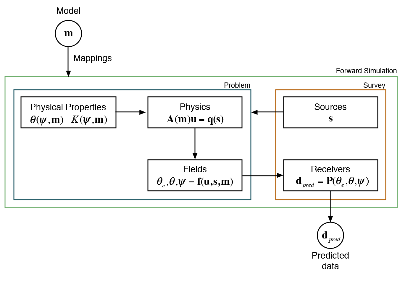
Figure C.1:The forward simulation framework that is used for Richards equation.
C.2.1Concepts
Here, we provide a brief overview of each of the components in the forward simulation. An in-depth discussion about each component in this framework has been published in the context of electromagnetic problems Heagy et al., 2016. Here, we present a succinct adaptation of this work in the context of the Richards equation by walking through Figure C.1. To compute pressure head responses everywhere in space and time, the forward simulation requires the definition of two physical property functions, which describe the water retention curve () and hydraulic conductivity function () on the simulation mesh. This method differs from many geophysical methods where physical properties are not dependent on the fields/fluxes (for example, electrical conductivity in direct current resistivity). Analogies exist here between induced polarization geophysical methods and the Richards equation, where the measured electrical conductivity depends upon the frequency of the alternating current. Regardless of the physics used, physical properties (or functions) must be defined throughout the computational domain. The physics defines the equation, in this case the Richards equation, which can be written as a matrix equation:
where is the solution of the matrix solve (possibly a field) and is both the right-hand side and the function of a source. In the time domain case, when backward Euler is used, amounts to a block bidiagonal matrix. The boundary conditions can be seen as sources, , when the discretization is written in weak-form (Section B.2.5). The sources must be included in both the physics and, in the case of electromagnetics, the fields. In the case of the Richards equations, the evaluation of the pressure head field to the water content field is dependent on the water retention curve, which may, in turn, depend on the model. These fields, defined everywhere in the computational domain, can be spatially and temporally interpolated onto the measurement locations of the receivers to create predicted data. In other geophysical methodologies, the data may be produced through a spatial or temporal derivative (e.g. gravity gradiometry), a potential difference (e.g. direct current resistivity), or a ratio involving multiple geophysical fields (e.g. magnetotellurics). Figure C.1 shows the conceptual steps involved in going from a model vector to predicted data. Heagy et al. (2016) discusses some additional intricacies; however, this conceptual organization into modular, exchangeable, and testable components is helpful when tackling the implicit derivatives necessary in the inverse problem.
C.2.2Derivatives
The process we follow to compute matrix-vector products with the sensitivity is shown in Figure C.2, where is built in stages by taking matrix vector products with the relevant derivatives in each component. This process is shown schematically in Figure C.2 for both and . As an example, let us consider our model to be the van Genuchten parameter, , which is defined as a heterogeneous parameter inside the computational domain. In this case, and no other parameters are considered to be active. The sensitivity of the forward simulation to the model takes the form:
The annotations in Figure C.2 denote which of the elements shown are responsible for computing the respective contribution to the sensitivity. If the model provided is instead in terms of , this property replaces the role of . The flexibility to invoke distinct properties of interest (e.g. , , source location, etc.) in the inversion requires quite a bit of 'wiring' to keep track of which model parameters are associated with which properties (physical properties, location properties, boundary conditions, etc.); this 'wiring' is achieved through a general Wires class that keeps track of the connections between properties and the model (Program C.2).
Although typically the source terms do not have model dependence and thus their derivatives are zero, the derivatives of must be considered in a general implementation Heagy et al., 2016. For example, if one wishes to use a nested approach, where source fields or boundary conditions are constructed by solving a simplified or different physics problem, the source terms may have dependance on the model. The source terms' dependance on the model means that their derivatives have a non-zero contribution to the sensitivity (cf. Haber (2015)Heagy et al. (2015)Heagy et al. (2016)).
The derivative of the solution, vector with respect to the model, is found by implicitly taking the derivative of the physics with respect to , giving:
The annotations below the equation indicate the methods of the Problem class that are responsible for calculating the respective derivatives. If multiple physical properties are internal to the , then this is indicated by an underscore in the method name (getADeriv_sigma). Typically the model dependence of the system matrix is through the physical properties. (for example, , in electromagnetics or , , and other van Genuchten parameters in the Richards equation). Thus, to compute derivatives with respect to , we first take the derivatives with respect to and we treat the dependence of on using chain rule.
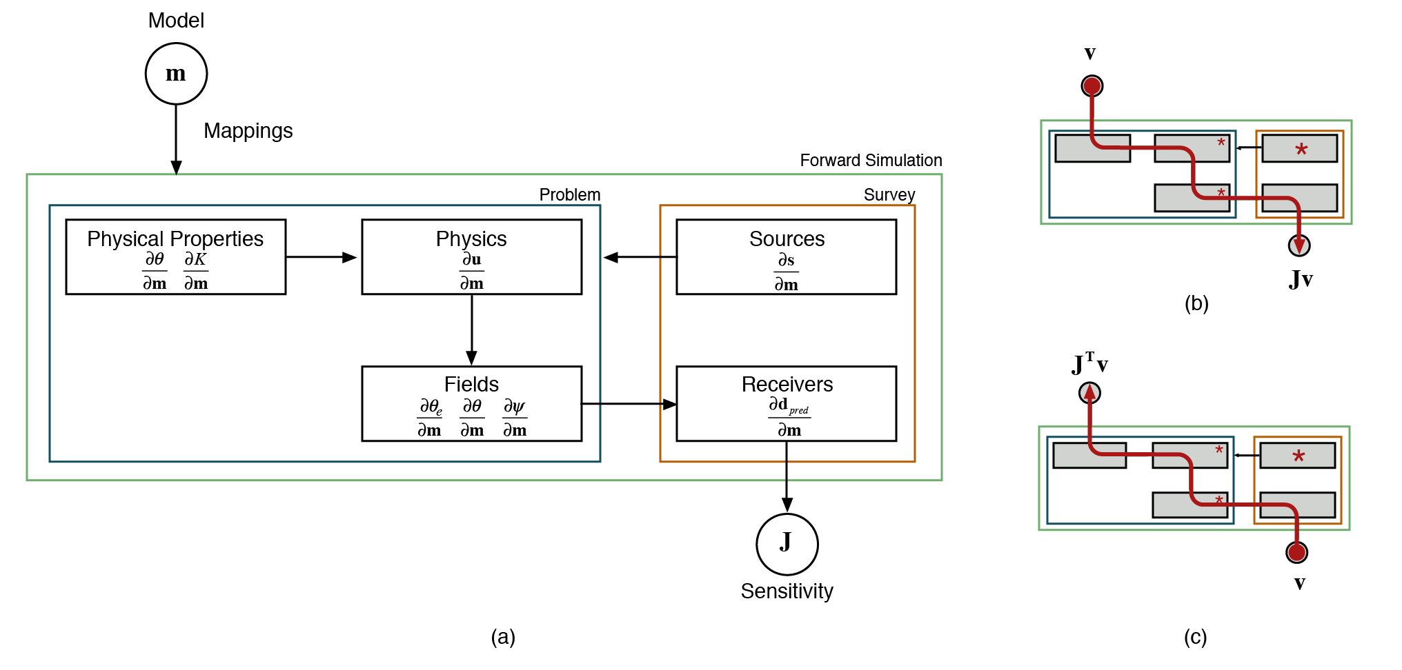
Figure C.2:The components required in calculating the derivatives of the forward simulation, showing (a) the modular nature of each derivative; (b) the process of multiplying each derivative in the forward sense with ; and (c) in the adjoint sense with .
C.2.3Properties and Mappings
Often, in solving an inverse problem, the model which we choose to invert for (the vector ) is some discrete representation of the earth that is decoupled from the physical property model or perhaps represents multiple physical properties. This decoupling requires the definition of a Mapping that is capable of translating to physical properties on the simulation mesh. For instance, if the inversion model is chosen to be log-conductivity, an exponential mapping is required to obtain electrical conductivity (i.e. ). To support this abstraction and integration to model conceptualization, the framework defines a number of extensible Mapping classes Cockett et al., 2015Kang et al., 2015Heagy et al., 2016. These Mappings must also be able to deal with the potential for multiple physical properties, potentially in different locations, in the forward simulation framework. For example, in the Richards equation, the water retention function is required in both the physics and the fields to translate pressure head to water content or saturation. As we are in the process of developing a computational ontology that is extensible and applicable across disciplines, our framework is explicit about where the physical properties (or functions and their properties) are involved in the forward simulation framework. For example, in Program~\ref{program:properties}, we can define a base class that represents the hydraulic conductivity function. Many variants (subclasses) of this function exist, which define parameters in different ways, including van Genuchten, Brooks-Corey, splines, interpolation, etc. The properties on these subclasses are the parameters that one might be interested in inverting for (in van Genuchten, these would include , , , and ). The Problem class, which contains the physics, can declaratively define that it requires a valid instance of a hydraulic conductivity function. This inheritance is similar for the water retention, which can be defined on both the problem and the fields. The declarative nature of these properties is the backbone of extracting an ontology, which can be used in a variety of other ways (specification, search, documentation, collaboration, etc.). In defining the properties, we also define a map, , to that property as well as a derivative with respect to the model.
import properties
from SimPEG import Props, Problem


class HydraulicConductivity(Props.HasModel):
    """The base hydraulic conductivity function"""


class Vangenuchten_k(HydraulicConductivity):

    Ks, KsMap, KsDeriv = Props.Invertible(
        "Saturated hydraulic conductivity",
        default=1e3
    )

    alpha, alphaMap, alphaDeriv = Props.Invertible(
        "inverse of the air entry suction [L-1]",
        default=6.0, min=0
    )


class BrooksCorey_k(HydraulicConductivity):
    """Or a spline, or something custom"""


class RichardsProblem(Problem.BaseTimeProblem):

    hydraulic_conductivity = properties.Instance(
        'hydraulic conductivity function',
        HydraulicConductivity
    )
Program C.1:Definition of a hydraulic conductivity model with multiple invertible properties that is declaratively attached to the Richards problem class.
The mappings from the model space to a physical property on the computational domain are a key way to interface to domain knowledge in other disciplines (e.g. structural geology). Additionally, they allow the inversion methodology to turn on or off sensitivity to the model at a property by property basis; this is completed by a Wires utility, which creates projection matrices that sample the model vector at the appropriate location(s). Program C.2 demonstrates this utility in Python code and shows the outcome of assumptions using assert statements. In this case, we define the model vectors to be and and use the wires to attach these vectors to the physical properties. In the inversion, however, we may wish to invert in log conductivity space for , as this property varies logarithmically rather than linearly. To do this, we use an additional Mapping to take the exponential of the model before setting the parameter in the hydraulic conductivity function. The length of these transformations is arbitrary and extremely specific to the case study or geoscience hypothesis (e.g. survey design, parametric inversions, or sensitivity analysis). The mappings between model conceptualization and physical properties can be broken into composable, reusable pieces, which can use the chain rule to evaluate the derivative of the transformation. Figure C.3 shows this evaluation in action, where a logarithmically scaled conductivity in a layered earth is transformed into the physical property on the entire computational domain.
import numpy as np
from SimPEG import Mesh, Maps
from SimPEG.FLOW.Richards import Empirical

mesh = Mesh.TensorMesh([[(1, 40)]], 'N')            # Create mesh with 40 cells
k_fun, theta_fun = Empirical.van_genuchten(mesh)    # Create empirical models

k_sat = 1e-3                                        # Define homogeneous physical properties
alpha = 6.0

k_sat_model = [np.log(k_sat)]*mesh.nC               # Put values into array, log(Ks) is the model
alpha_model = [alpha]*mesh.nC
model = np.array(k_sat_model + alpha_model)

assert len(model) == mesh.nC * 2                    # We have 80 model parameters

theta_r = np.array([0.02]*mesh.nC)                  # Define other properties (not in model)
theta_s = np.array([0.30]*mesh.nC)

wires = Maps.Wires(                                 # Create wires from model to properties
    ('Ks', mesh.nC),                                # $K_s$ gets 40 parameters
    ('alpha', mesh.nC)                              # $\alpha$ gets 40 parameters
)

# Use the maps to define Ks and alpha
k_fun.KsMap = Maps.ExpMap(mesh) * wires.Ks          # Add the exponential mapping
k_fun.alphaMap = theta_fun.alphaMap = wires.alpha   # Note that alpha is in both functions

theta_fun.theta_r = theta_r                         # Use the properties to define $\theta_r$ & $\theta_s$
theta_fun.theta_s = theta_s

k_fun.model = theta_fun.model = model               # Set the model for each function

# Test the setup of the functions
assert np.isclose(k_fun.alpha[0], alpha)            # Check that the mappings are working
assert np.isclose(theta_fun.alpha[0], alpha)
assert np.isclose(k_fun.Ks[0], k_sat)               # Including the exponential
assert k_fun.KsDeriv.shape == (40, 80)              # Check the $K_s$ derivative is the correct shape
assert theta_fun.theta_rMap is None                 # Check that there are no Maps for $\theta_r$
assert theta_fun.theta_sMap is None                 # Nor for $\theta_s$
assert theta_fun.theta_rDeriv == 0                  # Which means the derivative, $\frac{\partial \theta_r}{\partial \mathbf{m}}$, is zero

print(k_fun.summary())                              # Print a summary of the function

# >> Physical Properties:
# >>  [*] I: set by default value
# >>  [*] Ks: set by the `KsMap`: ComboMap[ExpMap(40,40) * Projection(40,80)] * model(80)
# >>  [*] alpha: set by the `alphaMap`: Projection(40,80) * model(80)
# >>  [*] n: set by default value
Program C.2:Demonstration of the ability to choose arbitrary parameters to include in a model, and use the chain rule to compose parameterizations.
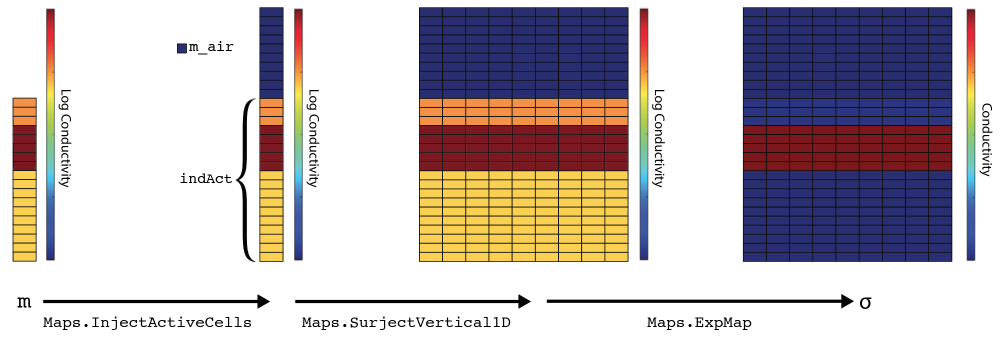
Figure C.3:Mapping an inversion model, a 1D layered, log conductivity model defined below the surface, to electrical conductivity defined in the full simulation domain.
C.3Parameterizations
In the following case studies, I will touch briefly on some key questions and how the framework developed can answer these classes of questions. Many of the case studies have been published and represent collaborative work with many colleagues. In this section, rather than repeating the conclusion of each study, I will highlight what I have learned and how the framework developed can be used.
Some geoscience questions:
- What is the distribution of physical properties?
- What space?
- What about known distributions?
- What is the sensitivity to a conceptual model?
- For example, in survey design?
- How does this extend to structural geologic modelling?
- What is the dimensionality (1D, 2D, 3D, or 4D) of the problem?
- For example, in electromagnetics?
- How do we keep control variables when testing assumptions?
- How can we integrate, nest, couple, and join different problems?
- For example, in a primary secondary formulation?
- In the general case?
C.3.1Expected distributions
Electrical or hydraulic conductivity are often parameterized logarithmically. This logarithmic parameterization changes the space in which the inversion 'searches' for an answer to the optimization problem. In the Richards equation, for example, by choosing the parameterization of van Genuchten, we constrain the inversion to pulling only from a set of parameterizations of this function. In Heagy et al. (2014), we investigated two approaches for identifying the extent and location of an electrically conductive proppant. Hydraulic fracturing uses sand or ceramic beads to prop newly created fractures open; as such, the location of the proppant represents the volume of a reservoir that can be effectively drained. The standard approach involves using an uncoupled geophysical inversion to create an image of electrical conductivity and then, subsequently, interpret that distribution either qualitatively or quantitatively (Figure C.4). In Heagy et al. (2013), the authors investigated the geophysical responses of conductive and permeable proppant particles. Later research by Heagy lead to a parameterization using effective medium theory to analytically describe the relationship between conductivity and volume fraction of the proppant. In Heagy et al. (2014), we used this relation directly in a coupled geophysical inversion for the volume of the proppant. Furthermore, by parameterizing the inversion in terms of volume, rather than conductivity, we can use the known volume of the proppant pumped into the synthetic reservoir as another datum. This coupled methodology was tested on a synthetic example and the joint inversion of geophysical and volume data showed promising results.
This coupled geophysical method can be completed through a single, custom made Mapping that codifies the effective medium theory parameterization and the derivative. We can then attach this mapping to a physical property, such as electrical conductivity. By changing the space in which we choose to conceptualize the model, it is possible to add more a priori information and other datum.

Figure C.4:(a) Traditional approach to inversion, where the model space, electrical conductivity, is mapped to data space, the electromagnetic response, through a forward model. The inversion then provides a method by which we estimate a model that is consistent with the observed data. The recovered conductivity model is then used to infer information about the reservoir properties of interest, in this case, the distribution of proppant. (b) Parametrized inversion, where we parametrize the model space, electrical conductivity, in terms of the property of interest, the distribution of proppant. By defining such a parametrization, the inversion can provide a means of estimating the properties of interest directly from the data.
C.3.2Survey design
Heagy et al. (2016) presented the forward simulation framework for the context of electromagnetic simulations and inversions. One of the examples in this paper dealt with a steel-cased well, which was used to deliver a galvanic or inductive source to a target reservoir (Figure C.5). Here, we posed the question: How sensitive are the data to the location, depth, and conductivity of a target in a reservoir? To answer this question, we conceptualized a simple model of location, dimensions, and conductivities of an idealized block in a reservoir layer; all model parameters are visualized in Figure C.5. The challenge here is that the steel-cased well has a thickness on the order of millimeters, while being kilometers long. Tackling this challenge in a computationally efficient manner required a primary-secondary approach, where source fields were constructed by solving a simplified problem without the target on a cylindrically symmetric mesh. However, this approach required that the contribution of the model sensitivity had to be efficiently traced all the way back through the primary fields. Figure C.5 shows the nesting of two forward modelling frameworks. By looking at the sensitivity to these model parameters, the paper drew conclusions about potential survey designs and to what extent the conceptual model could be resolved by noisy data.
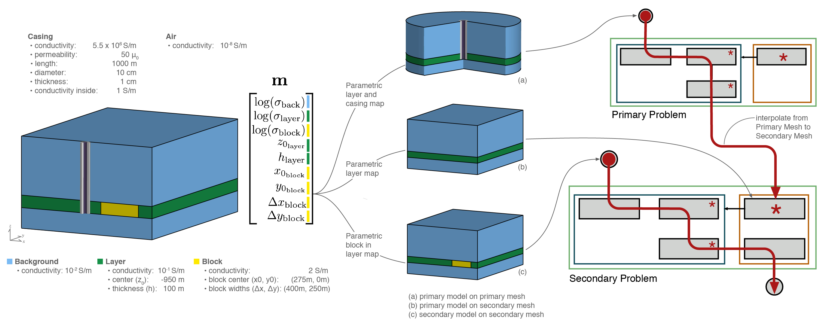
Figure C.5:Setup of a parametric models for a steel cased well and a reservoir target. The calculation of sensitivity for using a primary secondary approach is shown using the forward simulation framework.
This example required multiple formulations of Maxwell's equations on two different mesh types. The model could be conceptualized and potentially mapped to both electrical conductivity and magnetic permeability. The mappings required for this model conceptualization are largely reusable for other contexts. The sensitivity to the model parameters required that two problems be nested, which showed the value of composable pieces in a geophysical inversion framework.
C.3.3Geologic modeling
While completing my studies, I was involved in creating a number of structural geologic modelling tools Cockett et al., 2014Cockett, 2012Cockett, 2015Funning & Cockett, 2012Cockett et al., 2016Cockett, 2013. Over 300,000 people around the world have used these tools, primarily in introductory geoscience education Cockett et al., 2016. These tools allow rapid conceptual modelling of geologic scenarios (Figure C.6). Again, this process can be thought of as a mapping that codifies geologic knowledge and provides physical properties as a function of space. Using these mappings directly in an inversion, however, is difficult as the parameterization is spatially coupled; that is, a single parameter, such as rotation of a tilting event or period of a folding event, can change almost all physical properties at once. This spatial coupling is in contrast to a spatially decoupled voxel-based parameterization, where each cell centered parameter has no effect on its neighbours. Due to the spatial coupling, the explicit geologic parameterizations developed in Cockett et al., 2016 creates a non-convex objective function, which is difficult to minimize with deterministic optimization. Implicit geologic modelling, in contrast, solves an inverse problem by using radial basis functions to create a spatially extensive geologic parameterization (cf. Hillier et al. (2014)). Including this implicit modelling into the geophysics inversion framework as a mapping could be promising way to include geologic information.
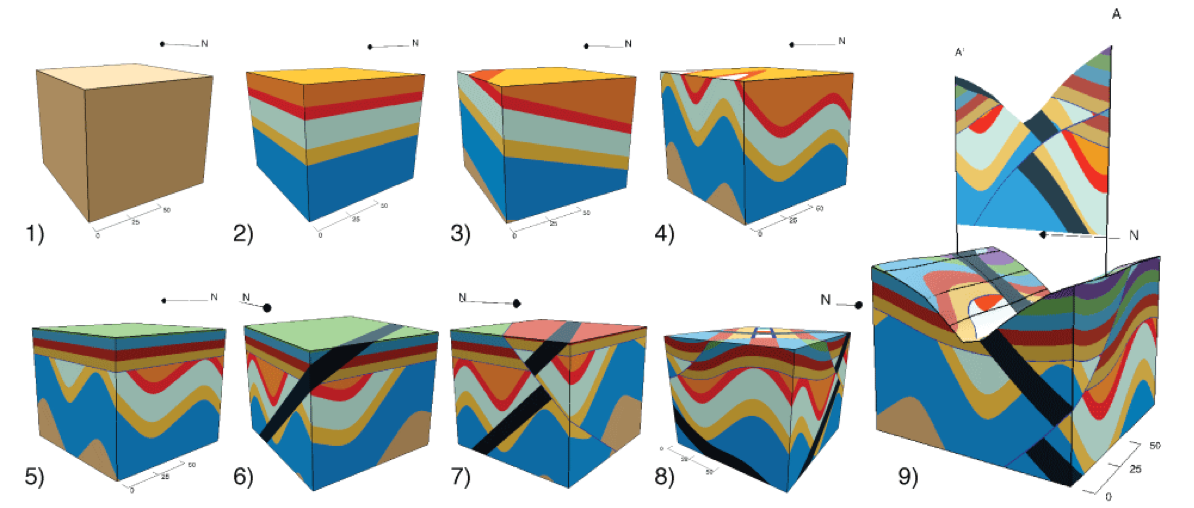
Figure C.6:Parameterized geologic models using a series of analytic functions. Models were created using Visible Geology (https://
C.3.4Dimensionality and controlled variables
In Kang et al. (2015), we explored the advantages to increasing the dimensionality of the physical problem being solved (in this case, ground loop, time domain electromagnetics). We explored these advantages over a three-dimensional synthetic model of seawater intrusion into a confined aquifer (Figure C.7). The experiment allowed for comparisons between the various dimensions because the tools were written in a consistent framework where only a single variable was changing at a time. The increased dimensionality, in this case, led to a better recovery of the seawater intrusion interface. Kang et al., 2014 subsequently fit the saltwater intrusion by a parametric surface. In Pidlisecky et al. (2013), however, we used a decrease in dimensionality (from 2.5D to 1D), which was tested for the ability to similarly fit collected data. In Heagy et al. (2016), data inversions were explored in both time domain and frequency domain electromagnetics. Figure C.8 shows the similarities between the two forward simulation frameworks. Although the internals of the implementation differ slightly, the inversion framework that we used is identical.
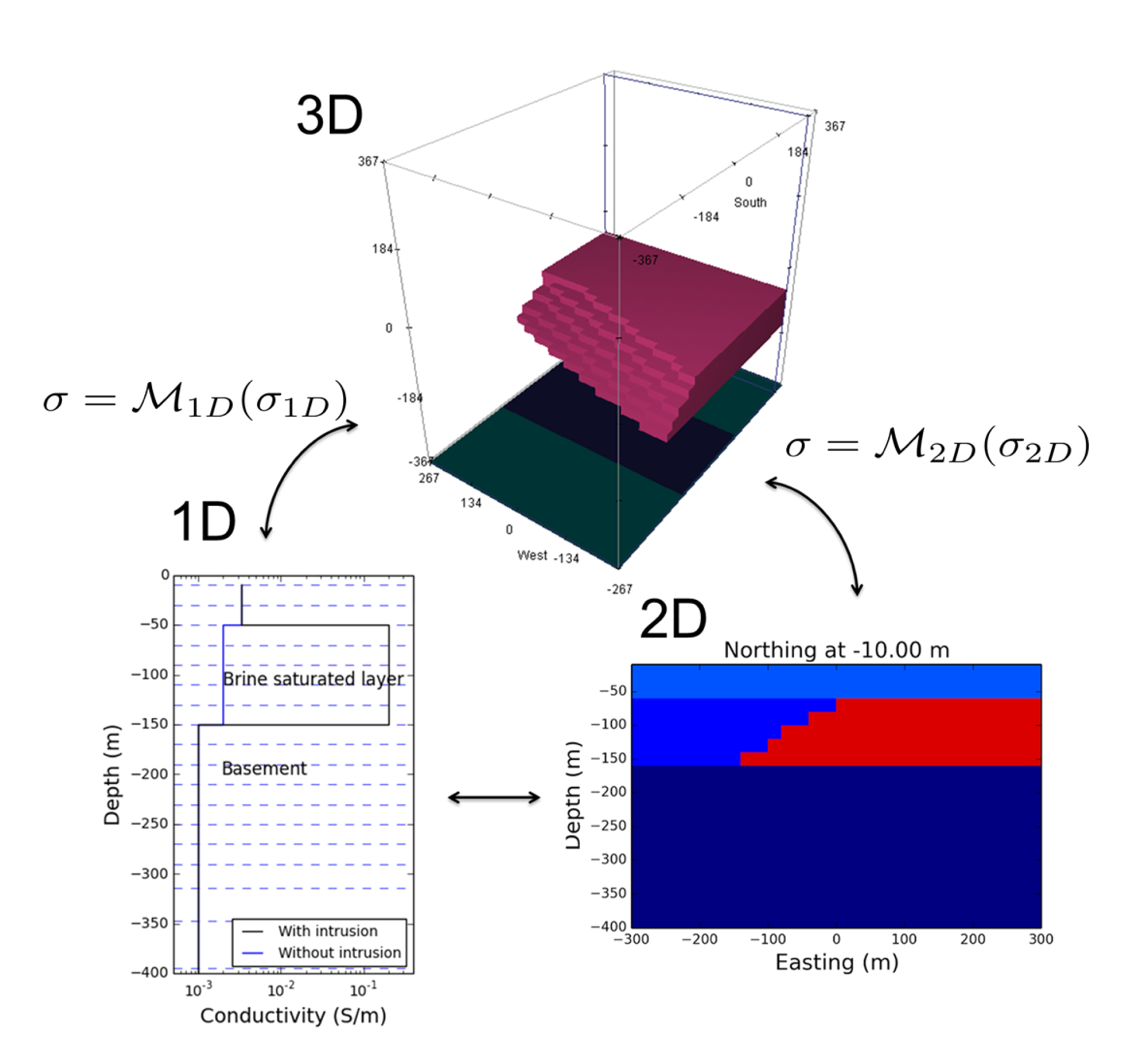
Figure C.7:Conceptual diagram of moving between 1D, 2D, and 3D models.
The flexibility to explore the dimensionality of the problem under consideration is important; this can be enabled by a consistent set of tools that allow you to control all variables except the dimensionality of the computational domain. When comparing between formulations of the same physics, the forward problems can inherit from and utilize many of the same components and the inversion machinery is identical. Rather than comparing inversion results to a completely different black-box implementation, these shared components of the framework promotes controlled variables and more rigorous comparisons of inversion methodologies across physical problems.
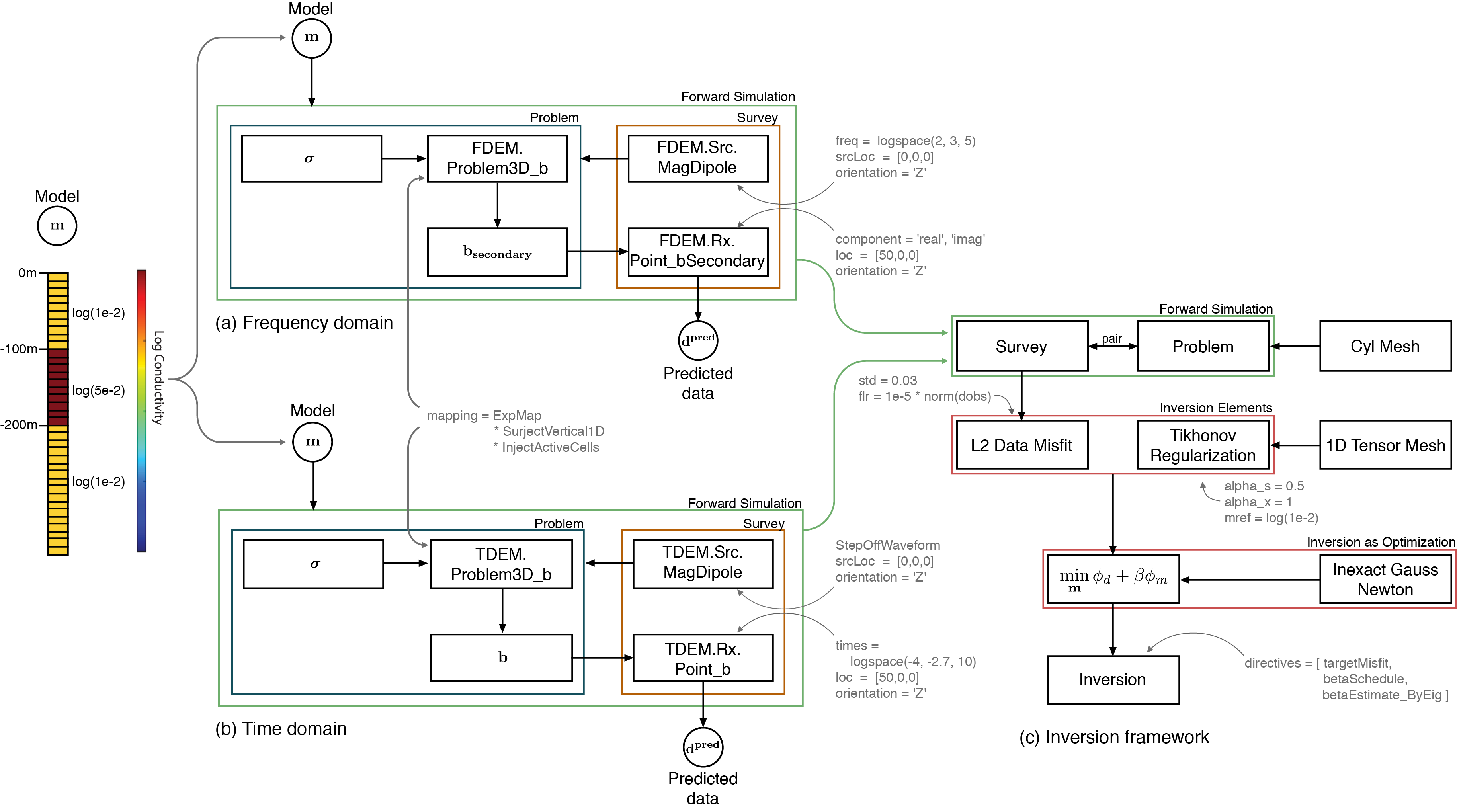
Figure C.8:Diagram showing the entire setup and organization of (a) the frequency domain simulation; (b) the time domain simulation; and (c) the common inversion framework used for each example. The muted text shows the programmatic inputs to each class instance.
C.3.5Nesting
There are many future research opportunities for combining, coupling, nesting, or otherwise integrating different physical problems. An example of these opportunities was completed in Heagy et al. (2016), where we nested a physics problem inside another one (Figure C.5). In this case, we nested the same physics problem; however, in Rosenkjaer et al. (2016), the authors used the framework to combine electromagnetic dipole sources with the magnetotelluric forward modelling to investigate coherent source interference. The growing field of hydrogeophysics will continue to combine geophysics and fluid flow problems; the use of a consistent and integrated framework should help to further these goals.
C.4Conclusions
Geologic and a priori assumptions are often given through parameterizations. The parameterizations necessary for a specific case study will often need to be unique to answer or predict a specific geoscience hypothesis. Through the exploration of numerous case studies across the geophysical, hydrologic, and geologic literature, we presented a forward modelling framework in Heagy et al. (2016). The important aspects of this framework are: (a) rigorously defining the properties that can be inverted for; (b) allowing these properties to be defined directly or wiring the property to the model through a mapping; and, (c) providing a number of extensible and reusable mapping components, which, when chained together, allow for efficient calculation of the sensitivity. The forward modelling framework presented maintains the computational scalability that is necessary to invert for large-scale 3D distributions of parameters (such as in electromagnetics or vadose zone flow). It is important to note that this framework also allows for customization through extensible mappings to custom model conceptualizations. By defining these components in a common framework, we enable hypothesis testing and exploration of assumptions by changing single variables (e.g. formulation or dimensionality) while keeping other variables controlled. The nesting and coupling of forward simulations, combined with these mappings between model conceptualizations, is important to any framework that aims to enhance quantitative geoscience collaboration.
- Williams, N. C. (2008). Geologically-constrained UBC–GIF Gravity And Magnetic Inversions With Examples From The Agnew-Wiluna Greenstone Belt, Western Australia [PhD]. University of British Columbia.
- Oldenburg, D. W., & Li, Y. (2005). Inversion for Applied Geophysics: A Tutorial. In Near-Surface Geophysics (pp. 89–150). 10.1190/1.9781560801719.ch5
- Li, Y., & Oldenburg, D. W. (1998). 3-D inversion of gravity data. Geophysics, 63(1), 109–119. 10.1190/1.1444302
- Li, Y., & Oldenburg, D. W. (1996). 3D Inversion of magnetic data. Geophysics, 61(2), 394–408.
- Pidlisecky, A., Haber, E., & Knight, R. (2007). RESINVM3D: A 3D resistivity inversion package. GEOPHYSICS, 72(2), H1–H10. 10.1190/1.2402499